Задача хищник жертва python

Lotka-Volterra equations¶

Also known as predator-prey equations, describe the variation in populations of two species which interact via predation. For example, wolves (predators) and deer (prey). This is a classical model to represent the dynamic of two populations.

Let \(\alpha>0\) , \(\beta>0\) , \(\delta>0\) and \(\gamma>0\) . The system is given by

Where \(x\) represents prey population and \(y\) predators population. It’s a system of first-order non-linear ordinary differential equations.

Problem reformulation¶

\[ \begin\begin\begin X = \begin x \\ y \end\end\\and rewrite so the problem above as\end\end \]
\[\begin\dot = \begin x (\alpha — \beta y) \\ y (-\delta + \gamma x) \end = f(X)\end\]

Remark : it’s an autonomous problem.

Numerical simulation¶

Settings¶

alpha = 1. #mortality rate due to predators beta = 1. delta = 1. gamma = 1. x0 = 4. y0 = 2. def derivative(X, t, alpha, beta, delta, gamma): x, y = X dotx = x * (alpha - beta * y) doty = y * (-delta + gamma * x) return np.array([dotx, doty]) 

Nt = 1000 tmax = 30. t = np.linspace(0.,tmax, Nt) X0 = [x0, y0] res = integrate.odeint(derivative, X0, t, args = (alpha, beta, delta, gamma)) x, y = res.T 

plt.figure() plt.grid() plt.title("odeint method") plt.plot(t, x, 'xb', label = 'Deer') plt.plot(t, y, '+r', label = "Wolves") plt.xlabel('Time t, [days]') plt.ylabel('Population') plt.legend() plt.show() 

IPython.core.display.Javascript object> 

import random import matplotlib.cm as cm 

betas = np.arange(0.9, 1.4, 0.1) nums=np.random.random((10,len(betas))) colors = cm.rainbow(np.linspace(0, 1, nums.shape[0])) # generate the colors for each data set fig, ax = plt.subplots(2,1) for beta, i in zip(betas, range(len(betas))): res = integrate.odeint(derivative, X0, t, args = (alpha,beta, delta, gamma)) ax[0].plot(t, res[:,0], color = colors[i], linestyle = '-', label = r"$\beta = $" + " ".format(beta)) ax[1].plot(t, res[:,1], color = colors[i], linestyle = '-', label = r" $\beta = $" + " ".format(beta)) ax[0].legend() ax[1].legend() ax[0].grid() ax[1].grid() ax[0].set_xlabel('Time t, [days]') ax[0].set_ylabel('Deer') ax[1].set_xlabel('Time t, [days]') ax[1].set_ylabel('Wolves'); 

IPython.core.display.Javascript object> 

Phase portrait¶

The phase portrait is a geometrical representation of the trajectories of a dynamical system in the phase space (axes corresponding to the state variables \(x\) and \(y\) ). It is a tool for visualizing and analyzing the behavior of dynamic systems. Particularly, in case of oscillatory systems like Lotka-Volterra equations.

plt.figure() IC = np.linspace(1.0, 6.0, 21) # initial conditions for deer population (prey) for deer in IC: X0 = [deer, 1.0] Xs = integrate.odeint(derivative, X0, t, args = (alpha, beta, delta, gamma)) plt.plot(Xs[:,0], Xs[:,1], "-", label = "$x_0 =$"+str(X0[0])) plt.xlabel("Deer") plt.ylabel("Wolves") plt.legend() plt.title("Deer vs Wolves"); 

IPython.core.display.Javascript object> 

Theses curves illustrate that the system is periodic because they are closed.

Solving with explicit Euler method

def Euler(func, X0, t, alpha, beta, delta, gamma): """ Euler solver. """ dt = t[1] - t[0] nt = len(t) X = np.zeros([nt, len(X0)]) X[0] = X0 for i in range(nt-1): X[i+1] = X[i] + func(X[i], t[i], alpha, beta, delta, gamma) * dt return X 

Xe = Euler(derivative, X0, t, alpha, beta, delta, gamma) plt.figure() plt.title("Euler method") plt.plot(t, Xe[:, 0], 'xb', label = 'Deer') plt.plot(t, Xe[:, 1], '+r', label = "Wolves") plt.grid() plt.xlabel("Time, $t$ [s]") plt.ylabel('Population') plt.ylim([0.,3.]) plt.legend(loc = "best") plt.show() 

IPython.core.display.Javascript object> 

plt.figure() plt.plot(Xe[:, 0], Xe[:, 1], "-") plt.xlabel("Deer") plt.ylabel("Wolves") plt.grid() plt.title("Phase plane : Deer vs Wolves (Euler)"); 

IPython.core.display.Javascript object> 

With RK4¶

def RK4(func, X0, t, alpha, beta, delta, gamma): """ Runge Kutta 4 solver. """ dt = t[1] - t[0] nt = len(t) X = np.zeros([nt, len(X0)]) X[0] = X0 for i in range(nt-1): k1 = func(X[i], t[i], alpha, beta, delta, gamma) k2 = func(X[i] + dt/2. * k1, t[i] + dt/2., alpha, beta, delta, gamma) k3 = func(X[i] + dt/2. * k2, t[i] + dt/2., alpha, beta, delta, gamma) k4 = func(X[i] + dt * k3, t[i] + dt, alpha, beta, delta, gamma) X[i+1] = X[i] + dt / 6. * (k1 + 2. * k2 + 2. * k3 + k4) return X 

Xrk4 = RK4(derivative, X0, t, alpha, beta, delta, gamma) plt.figure() plt.title("RK4 method") plt.plot(t, Xrk4[:, 0], 'xb', label = 'Deer') plt.plot(t, Xrk4[:, 1], '+r', label = "Wolves") plt.grid() plt.xlabel("Time, $t$ [s]") plt.ylabel('Population') plt.legend(loc = "best") plt.show(); 

IPython.core.display.Javascript object> 

plt.figure() plt.plot(Xrk4[:, 0], Xrk4[:, 1], "-") plt.xlabel("Deer") plt.ylabel("Wolves") plt.grid() plt.title("Phase plane : Deer vs Wolves (RK4)"); 

IPython.core.display.Javascript object> 

Источник

Matplotlib: lotka volterra tutorial¶

This example describes how to integrate ODEs with the scipy.integrate module, and how to use the matplotlib module to plot trajectories, direction fields and other information.

You can get the source code for this tutorial here: tutorial_lokta-voltera_v4.py.

Presentation of the Lotka-Volterra Model¶

We will have a look at the Lotka-Volterra model, also known as the predator-prey equations, which is a pair of first order, non-linear, differential equations frequently used to describe the dynamics of biological systems in which two species interact, one a predator and the other its prey. The model was proposed independently by Alfred J. Lotka in 1925 and Vito Volterra in 1926, and can be described by

with the following notations:

• u: number of preys (for example, rabbits)
• v: number of predators (for example, foxes)
• a, b, c, d are constant parameters defining the behavior of the population:
  • a is the natural growing rate of rabbits, when there’s no fox
  • b is the natural dying rate of rabbits, due to predation
  • c is the natural dying rate of fox, when there’s no rabbit
  • d is the factor describing how many caught rabbits let create a new fox

  We will use X=[u, v] to describe the state of both populations.

  Definition of the equations:

  #!python from numpy import * import pylab as p # Definition of parameters a = 1. b = 0.1 c = 1.5 d = 0.75 def dX_dt(X, t=0): """ Return the growth rate of fox and rabbit populations. """ return array([ a*X[0] - b*X[0]*X[1] , -c*X[1] + d*b*X[0]*X[1] ]) 

  Population equilibrium¶

  Before using !SciPy to integrate this system, we will have a closer look at position equilibrium. Equilibrium occurs when the growth rate is equal to 0. This gives two fixed points:

  #!python X_f0 = array([ 0. , 0.]) X_f1 = array([ c/(d*b), a/b]) all(dX_dt(X_f0) == zeros(2) ) and all(dX_dt(X_f1) == zeros(2)) # => True 

  Stability of the fixed points¶

  Near these two points, the system can be linearized: dX_dt = A_f*X where A is the Jacobian matrix evaluated at the corresponding point. We have to define the Jacobian matrix:

  #!python def d2X_dt2(X, t=0): """ Return the Jacobian matrix evaluated in X. """ return array([[a -b*X[1], -b*X[0] ], [b*d*X[1] , -c +b*d*X[0]] ]) 

  So near X_f0, which represents the extinction of both species, we have:

  #! python A_f0 = d2X_dt2(X_f0) # >>> array([[ 1. , -0. ], # [ 0. , -1.5]]) 

  Near X_f0, the number of rabbits increase and the population of foxes decrease. The origin is therefore a saddle point.

  #!python A_f1 = d2X_dt2(X_f1) # >>> array([[ 0. , -2. ], # [ 0.75, 0. ]]) # whose eigenvalues are +/- sqrt(c*a).j: lambda1, lambda2 = linalg.eigvals(A_f1) # >>> (1.22474j, -1.22474j) # They are imaginary numbers. The fox and rabbit populations are periodic as follows from further # analysis. Their period is given by: T_f1 = 2*pi/abs(lambda1) # >>> 5.130199 

  Integrating the ODE using scipy.integrate¶

  Now we will use the scipy.integrate module to integrate the ODEs. This module offers a method named odeint, which is very easy to use to integrate ODEs:

  #!python from scipy import integrate t = linspace(0, 15, 1000) # time X0 = array([10, 5]) # initials conditions: 10 rabbits and 5 foxes X, infodict = integrate.odeint(dX_dt, X0, t, full_output=True) infodict['message'] # >>> 'Integration successful.' 

  `infodict` is optional, and you can omit the `full_output` argument if you don’t want it. Type «info(odeint)» if you want more information about odeint inputs and outputs.

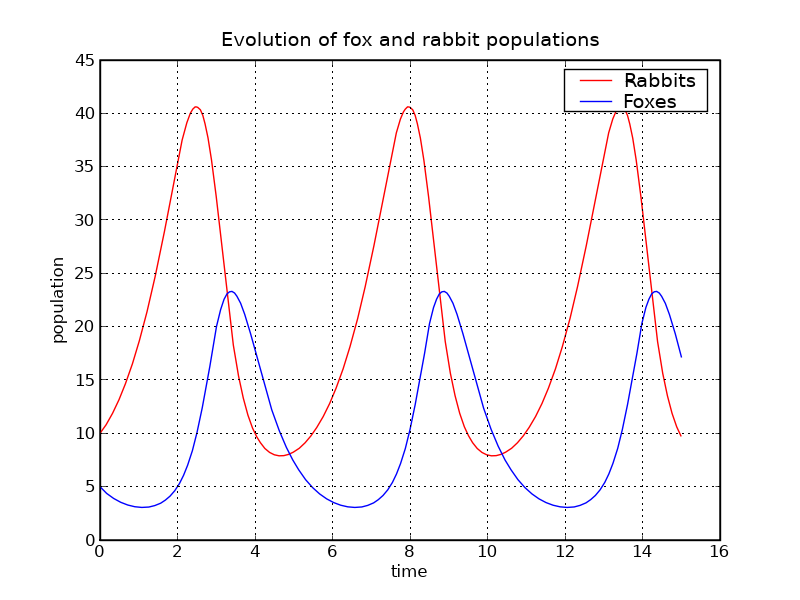
  We can now use Matplotlib to plot the evolution of both populations:

  #!python rabbits, foxes = X.T f1 = p.figure() p.plot(t, rabbits, 'r-', label='Rabbits') p.plot(t, foxes , 'b-', label='Foxes') p.grid() p.legend(loc='best') p.xlabel('time') p.ylabel('population') p.title('Evolution of fox and rabbit populations') f1.savefig('rabbits_and_foxes_1.png') 

  

  The populations are indeed periodic, and their period is close to the value T_f1 that we computed.

  Plotting direction fields and trajectories in the phase plane¶

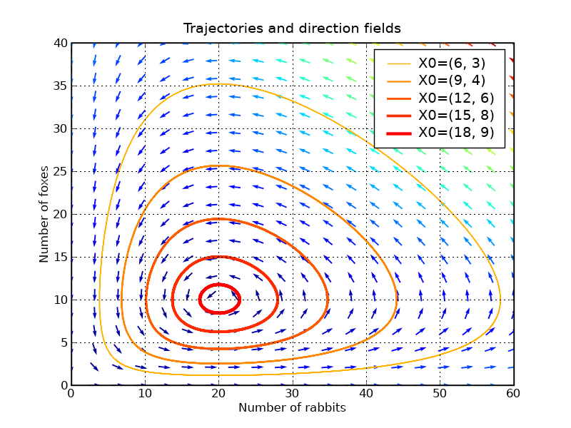
  We will plot some trajectories in a phase plane for different starting points between X_f0 and X_f1.

  We will use Matplotlib’s colormap to define colors for the trajectories. These colormaps are very useful to make nice plots. Have a look at ShowColormaps if you want more information.

  values = linspace(0.3, 0.9, 5) # position of X0 between X_f0 and X_f1 vcolors = p.cm.autumn_r(linspace(0.3, 1., len(values))) # colors for each trajectory f2 = p.figure() #------------------------------------------------------- # plot trajectories for v, col in zip(values, vcolors): X0 = v * X_f1 # starting point X = integrate.odeint( dX_dt, X0, t) # we don't need infodict here p.plot( X[:,0], X[:,1], lw=3.5*v, color=col, label='X0=(%.f, %.f)' % ( X0[0], X0[1]) ) #------------------------------------------------------- # define a grid and compute direction at each point ymax = p.ylim(ymin=0)[1] # get axis limits xmax = p.xlim(xmin=0)[1] nb_points = 20 x = linspace(0, xmax, nb_points) y = linspace(0, ymax, nb_points) X1 , Y1 = meshgrid(x, y) # create a grid DX1, DY1 = dX_dt([X1, Y1]) # compute growth rate on the gridt M = (hypot(DX1, DY1)) # Norm of the growth rate M[ M == 0] = 1. # Avoid zero division errors DX1 /= M # Normalize each arrows DY1 /= M #------------------------------------------------------- # Drow direction fields, using matplotlib 's quiver function # I choose to plot normalized arrows and to use colors to give information on # the growth speed p.title('Trajectories and direction fields') Q = p.quiver(X1, Y1, DX1, DY1, M, pivot='mid', cmap=p.cm.jet) p.xlabel('Number of rabbits') p.ylabel('Number of foxes') p.legend() p.grid() p.xlim(0, xmax) p.ylim(0, ymax) f2.savefig('rabbits_and_foxes_2.png') 

  

  This graph shows us that changing either the fox or the rabbit population can have an unintuitive effect. If, in order to decrease the number of rabbits, we introduce foxes, this can lead to an increase of rabbits in the long run, depending on the time of intervention.

  Plotting contours¶

  We can verify that the function IF defined below remains constant along a trajectory:

  #!python def IF(X): u, v = X return u**(c/a) * v * exp( -(b/a)*(d*u+v) ) # We will verify that IF remains constant for different trajectories for v in values: X0 = v * X_f1 # starting point X = integrate.odeint( dX_dt, X0, t) I = IF(X.T) # compute IF along the trajectory I_mean = I.mean() delta = 100 * (I.max()-I.min())/I_mean print 'X0=(%2.f,%2.f) => I ~ %.1f |delta = %.3G %%' % (X0[0], X0[1], I_mean, delta) # >>> X0=( 6, 3) => I ~ 20.8 |delta = 6.19E-05 % # X0=( 9, 4) => I ~ 39.4 |delta = 2.67E-05 % # X0=(12, 6) => I ~ 55.7 |delta = 1.82E-05 % # X0=(15, 8) => I ~ 66.8 |delta = 1.12E-05 % # X0=(18, 9) => I ~ 72.4 |delta = 4.68E-06 % 

  Plotting iso-contours of IF can be a good representation of trajectories, without having to integrate the ODE

  #!python #------------------------------------------------------- # plot iso contours nb_points = 80 # grid size x = linspace(0, xmax, nb_points) y = linspace(0, ymax, nb_points) X2 , Y2 = meshgrid(x, y) # create the grid Z2 = IF([X2, Y2]) # compute IF on each point f3 = p.figure() CS = p.contourf(X2, Y2, Z2, cmap=p.cm.Purples_r, alpha=0.5) CS2 = p.contour(X2, Y2, Z2, colors='black', linewidths=2. ) p.clabel(CS2, inline=1, fontsize=16, fmt='%.f') p.grid() p.xlabel('Number of rabbits') p.ylabel('Number of foxes') p.ylim(1, ymax) p.xlim(1, xmax) p.title('IF contours') f3.savefig('rabbits_and_foxes_3.png') p.show() 

  Источник

  Читайте также:  Java является императивным языком программирования