DataTechNotes
XGBoost stands for «Extreme Gradient Boosting» and it is an implementation of gradient boosting trees algorithm. The XGBoost is a popular supervised machine learning model with characteristics like computation speed, parallelization, and performance. You can find more about the model in this link.
- Preparing the data
- Defining and fitting the model
- Predicting and checking the results
- Video tutorial
- Source code listing
import xgboost as xgb from sklearn.datasets import load_boston from sklearn.model_selection import train_test_split from sklearn.model_selection import cross_val_score, KFold from sklearn.metrics import mean_squared_error import matplotlib.pyplot as plt
We use Boston house-price dataset as a regression dataset in this tutorial. After loading the dataset, first, we’ll separate data into x — feature and y — label. Then we’ll split them into the train and test parts. Here, I’ll extract 15 percent of the dataset as test data.
boston = load_boston() x, y = boston.data, boston.target xtrain, xtest, ytrain, ytest=train_test_split(x, y, test_size=0.15)
Defining and fitting the model
For the regression problem, we’ll use the XGBRegressor class of the xgboost package and we can define it with its default parameters. You can also set the new parameter values according to your data characteristics.
xgbr = xgb.XGBRegressor(verbosity=0)
XGBRegressor(base_score=0.5, booster='gbtree', colsample_bylevel=1, colsample_bynode=1, colsample_bytree=1, gamma=0, importance_type='gain', learning_rate=0.1, max_delta_step=0, max_depth=3, min_child_weight=1, missing=None, n_estimators=100, n_jobs=1, nthread=None, objective='reg:linear', random_state=0, reg_alpha=0, reg_lambda=1, scale_pos_weight=1, seed=None, silent=None, subsample=1, verbosity=1)
Next, we’ll fit the model with train data.
Predicting and checking the results
After training the model, we’ll check the model training score.
score = xgbr.score(xtrain, ytrain)
print("Training score: ", score)
Training score: 0.9738225090795732
We can also apply the cross-validation method to evaluate the training score.
scores = cross_val_score(xgbr, xtrain, ytrain,cv=10) print("Mean cross-validation score: %.2f" % scores.mean())
Mean cross-validataion score: 0.87
Or if you want to use the KFlold method in cross-validation it goes as below.
kfold = KFold(n_splits=10, shuffle=True) kf_cv_scores = cross_val_score(xgbr, xtrain, ytrain, cv=kfold ) print("K-fold CV average score: %.2f" % kf_cv_scores.mean())
K-fold CV average score: 0.87
Both methods show that the model is around 87 % accurate on average.
Next, we can predict test data, then check the prediction accuracy. Here, we’ll use MSE and RMSE as accuracy metrics.
ypred = xgbr.predict(xtest) mse = mean_squared_error(ytest, ypred) print("MSE: %.2f" % mse)
Finally, we’ll visualize the original and predicted test data in a plot to compare visually.
x_ax = range(len(ytest)) plt.plot(x_ax, ytest, label="original") plt.plot(x_ax, ypred, label="predicted")
plt.title("Boston test and predicted data") 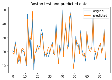
In this post, we’ve briefly learned how to build the XGBRegressor model and predict regression data in Python. The full source code is listed below.
import xgboost as xgb from sklearn.datasets import load_boston from sklearn.model_selection import train_test_split from sklearn.model_selection import cross_val_score, KFold from sklearn.metrics import mean_squared_error import matplotlib.pyplot as plt
boston = load_boston() x, y = boston.data, boston.target xtrain, xtest, ytrain, ytest = train_test_split(x, y, test_size=0.15) xgbr = xgb.XGBRegressor(verbosity=0) print(xgbr) xgbr.fit(xtrain, ytrain)
score = xgbr.score(xtrain, ytrain)
print("Training score: ", score)
# - cross validataion scores = cross_val_score(xgbr, xtrain, ytrain, cv=5) print("Mean cross-validation score: %.2f" % scores.mean()) kfold = KFold(n_splits=10, shuffle=True) kf_cv_scores = cross_val_score(xgbr, xtrain, ytrain, cv=kfold ) print("K-fold CV average score: %.2f" % kf_cv_scores.mean())
ypred = xgbr.predict(xtest) mse = mean_squared_error(ytest, ypred) print("MSE: %.2f" % mse) print("RMSE: %.2f" % (mse**(1/2.0))) x_ax = range(len(ytest)) plt.scatter(x_ax, ytest, s=5, color="blue", label="original") plt.plot(x_ax, ypred, lw=0.8, color="red", label="predicted") plt.legend() plt.show()
6 comments:
Hello,
I’ve a couple of question.
1. What are labels for x and y axis in the above graph?
2. Then I’m trying to understand the following example.
I’m confused about the first piece of code. It seems to me that cross-validation and Cross-validation with a k-fold method are performing the same actions. In the second example just 10 times more. The result is the same. I dont understand the cross-validation in first example what is for?
Thanks,
Marco Reply Delete

Hi,
1. The plot describes ‘medv’ column of boston dataset (original and predicted). x label is the number of sample and y label is the value of ‘medv’
2. They explain two ways of implementaion of cross-validation. You can use one of them.
how can write python code to upload similar work done like this in order to submit on kaggle.com. Thanks Reply Delete
Hi! Which version of scikit-learn and xgboost are you using? I am getting a weir error: KeyError ‘base_score’ Reply Delete
*******
kfold = KFold(n_splits=10, shuffle=True)
kf_cv_scores = cross_val_score(xgbr, xtrain, ytrain, cv=kfold )
print(«K-fold CV average score: %.2f» % kf_cv_scores.mean())
ypred = xgbr.predict(xtest)
********
imho, you cannot call predict() method just after calling cross_val_score() with xgbr object. That method makes a copy of the xgbr within and original xgbr stays unfitted (you still have to call xgbr.fit() method after using cross_val_score before using xgbr.predict(). Reply Delete
XGBoost for Regression
The results of the regression problems are continuous or real values. Some commonly used regression algorithms are Linear Regression and Decision Trees. There are several metrics involved in regression like root-mean-squared error (RMSE) and mean-squared-error (MSE). These are some key members of XGBoost models, each plays an important role.
- RMSE: It is the square root of mean squared error (MSE).
- MAE: It is an absolute sum of actual and predicted differences, but it lacks mathematically, that’s why it is rarely used, as compared to other metrics.
XGBoost is a powerful approach for building supervised regression models. The validity of this statement can be inferred by knowing about its (XGBoost) objective function and base learners. The objective function contains loss function and a regularization term. It tells about the difference between actual values and predicted values, i.e how far the model results are from the real values. The most common loss functions in XGBoost for regression problems is reg:linear, and that for binary classification is reg:logistics. Ensemble learning involves training and combining individual models (known as base learners) to get a single prediction, and XGBoost is one of the ensemble learning methods. XGBoost expects to have the base learners which are uniformly bad at the remainder so that when all the predictions are combined, bad predictions cancels out and better one sums up to form final good predictions. Code:
python3
Code: Linear base learner
python3
Note: The dataset needs to be converted into DMatrix. It is an optimized data structure that the creators of XGBoost made. It gives the package its performance and efficiency gains. The loss function is also responsible for analyzing the complexity of the model, and if the model becomes more complex there becomes a need to penalize it and this can be done using Regularization. It penalizes more complex models through both LASSO (L1) and Ridge (L2) regularization to prevent overfitting. The ultimate goal is to find simple and accurate models. Regularization parameters are as follows:
- gamma: minimum reduction of loss allowed for a split to occur. Higher the gamma, fewer the splits.
alpha: L1 regularization on leaf weights, larger the value, more will be the regularization, which causes many leaf weights in the base learner to go to 0. - lambda: L2 regularization on leaf weights, this is smoother than L1 and causes leaf weights to smoothly decrease, unlike L1, which enforces strong constraints on leaf weights.
Below are the formulas which help in building the XGBoost tree for Regression. Step 1: Calculate the similarity scores, it helps in growing the tree.
Similarity Score = (Sum of residuals)^2 / Number of residuals + lambda
Step 2: Calculate the gain to determine how to split the data.
Gain = Left tree (similarity score) + Right (similarity score) - Root (similarity score)
Step 3: Prune the tree by calculating the difference between Gain and gamma (user-defined tree-complexity parameter)
If the result is a positive number then do not prune and if the result is negative, then prune and again subtract gamma from the next Gain value way up the tree. Step 4: Calculate output value for the remaining leaves
Output value = Sum of residuals / Number of residuals + lambda
Note: If the value of lambda is greater than 0, it results in more pruning by shrinking the similarity scores and it results in smaller output values for the leaves. Let’s see a part of mathematics involved in finding the suitable output value to minimize the loss function For classification and regression, XGBoost starts with an initial prediction usually 0.5, as shown in the below diagram. 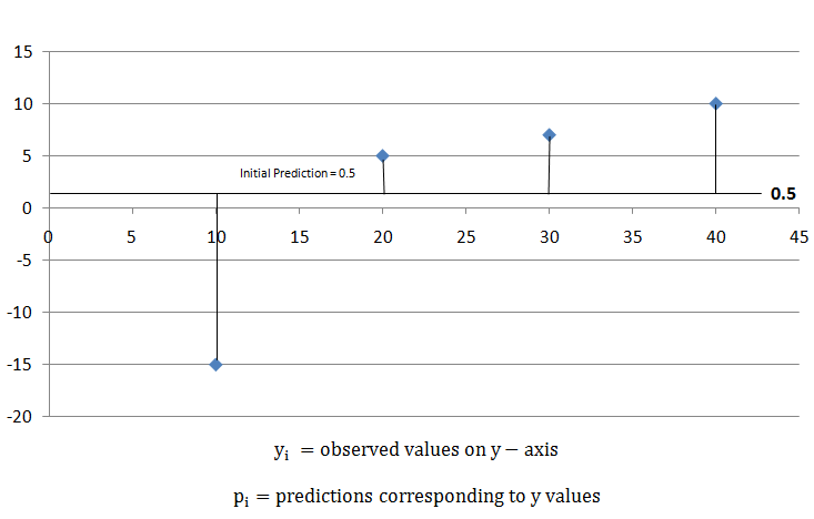 To find how good the prediction is, calculate the Loss function, by using the formula,
 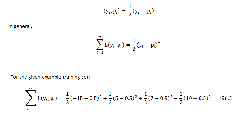 For the given example, it came out to be 196.5. Later, we can apply this loss function and compare the results, and check if predictions are improving or not. XGBoost uses those loss function to build trees by minimizing the below equation:
 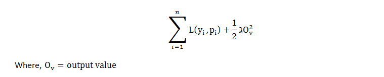 The first part of the equation is the loss function and the second part of the equation is the regularization term and the ultimate goal is to minimize the whole equation. For optimizing output value for the first tree, we write the equation as follows, replace p(i) with the initial predictions and output value and let lambda = 0 for simpler calculations. Now the equation looks like,
 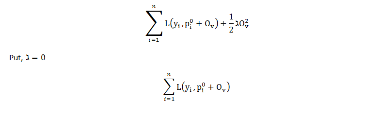 The loss function for initial prediction was calculated before, which came out to be 196.5. So, for output value = 0, loss function = 196.5. Similarly, if we plot the point for output value = -1, loss function = 203.5 and for output value = +1, loss function = 193.5, and so on for other output values and, if we plot this in the graph. we get a parabola like structure. This is the plot for the equation as a function of output values.
 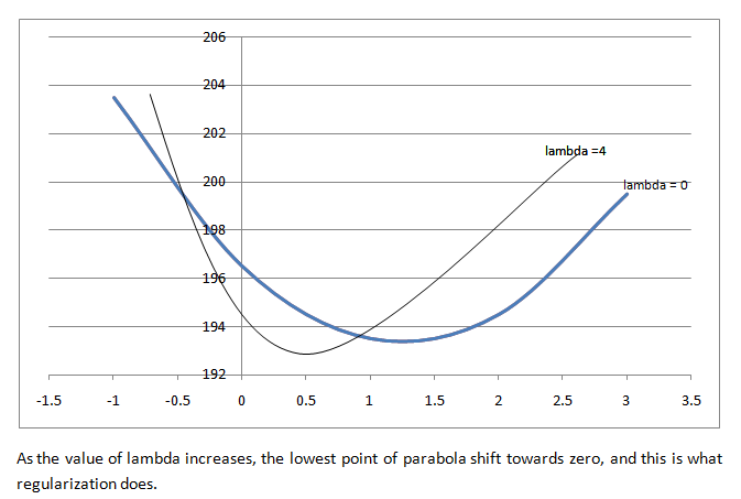 If lambda = 0, the optimal output value is at the bottom of the parabola where the derivative is zero. XGBoost uses Second-Order Taylor Approximation for both classification and regression. The loss function containing output values can be approximated as follows:
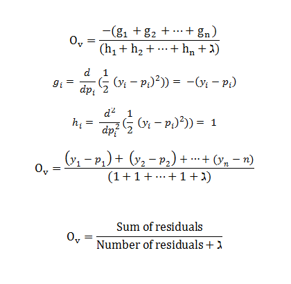
  The first part is Loss Function, the second part includes the first derivative of the loss function and the third part includes the second derivative of the loss function. The first derivative is related to Gradient Descent, so here XGBoost uses ‘g’ to represent the first derivative and the second derivative is related to Hessian, so it is represented by ‘h’ in XGBoost. Plugging the same in the equation:
 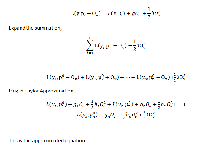 Remove the terms that do not contain the output value term, now minimize the remaining function by following steps:
- Take the derivative w.r.t output value.
- Set derivative equals 0 (solving for the lowest point in parabola)
- Solve for the output value.
- g(i) = negative residuals
- h(i) = number of residuals

This is the output value formula for XGBoost in Regression. It gives the x-axis coordinate for the lowest point in the parabola.
XGBoost Python Feature Walkthrough
This is a collection of examples for using the XGBoost Python package.