Центральная предельная теорема python

Central Limit Theorem Explained with Python Code

A simulation to explain Central Limit Theorem: even when a sample is not normally distributed, if you draw multiple samples and take each of their averages, these averages will represent a normal distribution.

All roads lead to Rome! Wait, no! All roads lead to Shibuya! Wait, no! All sample means lead to the population mean.

Central Limit Theorem suggests that if you randomly draw a sample of your customers, say 1000 customers, this sample itself might not be normally distributed. But if you now repeat the experiment say 100 times, then the 100 means of those 100 samples (of 1000 customers) will make up a normal distribution.

This line is important for us: ‘this sample itself might not be normally distributed’. Why? Because most things in life are not normally distributed; not grades, not wealth, not food, certainly not how much our customers pay in our shop. But everything in life has a Poisson distribution; better yet, everything in life can be explained by a Dirichlet distribution, but let’s stick with a Poisson for simplicity (Poisson is a simplified case of Dirichlet, in fact).

But actually in an e-commerce shop, most of our customers are non-buying customers. So the distribution actually looks like an exponential, and since a Poisson can be derived from an exponential, let’s make some exponential distributions to reflect our customers’ purchases.

Let’s Try an Example

Let us assume our customer base has an average order value of $170, so we will create exponential distributions with this average. We will attempt to get this value by looking at some sample averages.

Draw only four samples

Here, I draw a sample of 1000 customers. Then repeat this 4 times. I get the following four distributions (To get graphs similar to this, use the code at the end with repeat_sample_draws_exponential(4, 1000, 170, True) ):

And here is each of those 4 averages plotted (To get graphs similar to this, use the code at the end with…

Источник

Introduction to Central Limit Theorem: Examples, Calculation, Statistics in Python

The Central Limit Theorem (CLT) is often referred to as one of the most important theorems, not only in statistics but also in the sciences as a whole. In this blog, we will try to understand the essence of the Central Limit Theorem with simulations in Python.

• Samples and the Sampling Distribution
• What is the Central Limit Theorem?
• Central Limit Theorem — Statement & Assumptions
• Demonstration of CLT in action using simulations in Python with example
• Example 1 — Exponentially distributed population
• Example 2 — Binomially distributed population
• An Application of CLT in Investing/Trading
• The Challenge for Investors
• The Great Assumption of Normality in Finance
• The Shapiro-Wilk test
• The Role of Central Limit Theorem
• Testing Normality of Weekly and Monthly Returns
• Confidence Intervals

Samples and the Sampling Distribution

Before we get to the theorem itself, it is first essential to understand the building blocks and the context. The main goal of inferential statistics is to draw inferences about a given population, using only its subset, which is called the sample.

We do so because generally, the parameters which define the distribution of the population, such as the population mean \(\mu\) and the population variance \(\sigma^\), are not known.

In such situations, a sample is typically collected in a random fashion, and the information gathered from it is then used to derive estimates for the entire population.

The above-mentioned approach is both time-efficient and cost-effective for the organization/firm/researcher conducting the analysis. It is important that the sample is a good representation of the population, in order to generalize the inferences drawn from the sample to the population in any meaningful way.

The challenge though is that being a subset, the sample estimates are well, just estimates, and hence prone to error! That is, they may not reflect the population accurately.

For example, if we are trying to estimate the population mean \((\mu)\) using a sample mean \((\bar x)\), then depending on which observations land in the sample, we might get different estimates of the population with varying levels of errors.

What is the Central Limit Theorem?

The core point here is that the sample mean itself is a random variable, which is dependent on the sample observations.

Like any other random variable in statistics, the sample mean \((\bar x)\) also has a probability distribution, which shows the probability densities for different values of the sample mean.

This distribution is often referred to as the ‘sampling distribution’. The following diagram summarizes this point visually:

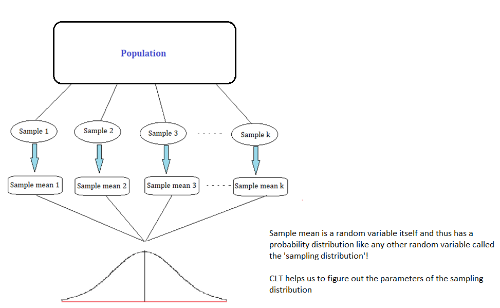
The Central Limit Theorem essentially is a statement about the nature of the sampling distribution of the sample mean under some specific condition, which we will discuss in the next section.

Central Limit Theorem — Statement & Assumptions

Suppose \(X\) is a random variable(not necessarily normal) representing the population data. And, the distribution of \(X\), has a mean of \(\mu\) and standard deviation \(\sigma\). Suppose we are taking repeated samples of size ‘n’ from the above population.

Then, the Central Limit Theorem states that given a high enough sample size, the following properties hold true:

• Sampling distribution’s mean = Population mean \((\mu)\), and
• Sampling distribution’s standard deviation (standard error) = \(\sigma/√n\), such that
• for n ≥ 30, the sampling distribution tends to a normal distribution for all practical purposes.

In the next section, we will try to understand the workings of the CLT with the help of simulations in Python.

Demonstration of CLT in action using simulations in Python with examples

The main point demonstrated in this section will be that for a population following any distribution, the sampling distribution (sample mean’s distribution) will tend to be normally distributed for large enough sample size.

We will consider two examples and check whether the CLT holds.

• Example 1 — Exponentially distributed population
• Example 2 — Binomially distributed population

Example 1 — Exponentially distributed population

Suppose we are dealing with a population which is exponentially distributed. Exponential distribution is a continuous distribution that is often used to model the expected time one needs to wait before the occurrence of an event.

The main parameter of exponential distribution is the ‘rate’ parameter \(\lambda\), such that both the mean and the standard deviation of the distribution are given by \((1/\lambda)\).

The following represents our exponentially distributed population:

E(X) = \(1/\lambda\) = \(\mu\)V(X) = \(1/\lambda^2\) = \(\sigma^2\), which means SD(X) = \(1/\lambda\) = \(\sigma\)

We can see that the distribution of our population is far from normal! In the following code, assuming that \(\lambda\)=0.25, we calculate the mean and the standard deviation of the population:

Population mean: 4.0 Population standard deviation: 4.0

Now we want to see how the sampling distribution looks for this population. We will consider two cases, i.e. with a small sample size (n= 2), and a large sample size (n=500).

First, we will draw 50 random samples from our population of size 2 each. The code to do the same in Python is given below:

sample 1	sample 2	sample 3	sample 4	sample 5	sample 6	sample 7	sample 8	sample 9	sample 10	.	sample 41	sample 42	sample 43	sample 44	sample 45	sample 46	sample 47	sample 48	sample 49	sample 50
x1	3.308423	7.105807	0.787859	2.811602	0.255161	5.085278	7.253975	2.549191	1.318133	0.659430	.	13.017465	10.280906	1.863208	4.000935	1.119582	1.640825	7.242127	0.807044	11.797688	4.585229
x2	2.969489	1.082994	3.382971	3.474494	8.949835	0.993594	7.335135	5.529222	3.760836	1.690919	.	8.690013	1.468530	0.376954	0.167118	4.100110	0.255927	1.754906	3.647159	1.883523	1.101046

Источник