Сигмоидная функция активации python

Функция сигмоидной активации – Реализация Python

Функция активации – это математическая функция, управляющая выходом нейронной сети. Функции активации помогают определить, будет ли нейрон уволить или нет.

Некоторые из популярных функций активации:

• Бинарный шаг
• Линейный
• Сигмоид
• Усадьба
• Relu.
• Утечка RELU.
• Софтмакс

Активация несет ответственность за добавление нелинейность к выходу модели нейронной сети. Без функции активации нейронная сеть – это просто линейная регрессия.

Математическое уравнение для расчета выхода нейронной сети:

В этом руководстве мы сосредоточимся на Сигмоидная функция активации. Эта функция поступает из функции Sigmoid в математике.

Давайте начнем с обсуждения формулы для функции.

Формула для функции активации сигмоидной активации

Математически вы можете представлять функцию активации Sigmoid AS:

Вы можете видеть, что знаменатель всегда будет больше 1, поэтому вывод всегда будет от 0 до 1.

Реализация функции активации Sigmoid в Python

В этом разделе мы узнаем, как реализовать функцию активации Sigmoid в Python.

Мы можем определить функцию в Python AS:

import numpy as np def sig(x): return 1/(1 + np.exp(-x))

Давайте попробуем запустить функцию на некоторых входах.

import numpy as np def sig(x): return 1/(1 + np.exp(-x)) x = 1.0 print('Applying Sigmoid Activation on (%.1f) gives %.1f' % (x, sig(x))) x = -10.0 print('Applying Sigmoid Activation on (%.1f) gives %.1f' % (x, sig(x))) x = 0.0 print('Applying Sigmoid Activation on (%.1f) gives %.1f' % (x, sig(x))) x = 15.0 print('Applying Sigmoid Activation on (%.1f) gives %.1f' % (x, sig(x))) x = -2.0 print('Applying Sigmoid Activation on (%.1f) gives %.1f' % (x, sig(x)))

Applying Sigmoid Activation on (1.0) gives 0.7 Applying Sigmoid Activation on (-10.0) gives 0.0 Applying Sigmoid Activation on (0.0) gives 0.5 Applying Sigmoid Activation on (15.0) gives 1.0 Applying Sigmoid Activation on (-2.0) gives 0.1

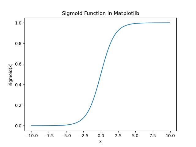
Построение сигмовидной активации с помощью Python

Чтобы с участием сигмовидной активации мы будем использовать Numpy Library:

import numpy as np import matplotlib.pyplot as plt x = np.linspace(-10, 10, 50) p = sig(x) plt.xlabel("x") plt.ylabel("Sigmoid(x)") plt.plot(x, p) plt.show()

Мы видим, что вывод составляет от 0 до 1.

Сигмовидная функция обычно используется для прогноз вероятностей, поскольку вероятность всегда от 0 до 1.

Одним из недостатков сигмоидной функции является то, что к конечным областям Значения Y реагируют очень меньше к изменению значений X.

Это приводит к проблеме, известной как исчезающий градиент проблема.

Исчезающий градиент замедляет процесс обучения и, следовательно, нежелательно.

Давайте обсудим некоторые альтернативы, которые преодолевают эту проблему.

Функция активации RELU

Лучшая альтернатива, которая решает эту проблему исчезновения градиента, – это функция активации RELU.

Функция активации RELU возвращает 0, если вход отрицательна иначе, возвращает ввод ввода.

Математически это представлено как:

Вы можете реализовать его в Python следующим образом:

Давайте посмотрим, как это работает на некоторых входах.

def relu(x): return max(0.0, x) x = 1.0 print('Applying Relu on (%.1f) gives %.1f' % (x, relu(x))) x = -10.0 print('Applying Relu on (%.1f) gives %.1f' % (x, relu(x))) x = 0.0 print('Applying Relu on (%.1f) gives %.1f' % (x, relu(x))) x = 15.0 print('Applying Relu on (%.1f) gives %.1f' % (x, relu(x))) x = -20.0 print('Applying Relu on (%.1f) gives %.1f' % (x, relu(x)))

Applying Relu on (1.0) gives 1.0 Applying Relu on (-10.0) gives 0.0 Applying Relu on (0.0) gives 0.0 Applying Relu on (15.0) gives 15.0 Applying Relu on (-20.0) gives 0.0

Проблема с RELU состоит в том, что градиент отрицательных входов выходит на нулю.

Это снова приводит к проблеме исчезновения градиента (нулевой градиент) для отрицательных входов.

Чтобы решить эту проблему, у нас есть еще одна альтернатива, известная как Элезначная функция активации RELU.

Элексиновая функция активации RELU

Утечки RELU обращаются к проблеме нулевых градиентов для отрицательного значения, давая чрезвычайно небольшой линейный компонент X к отрицательным входам.

Математически мы можем определить его как:

Вы можете реализовать его в Python, используя:

def leaky_relu(x): if x>0 : return x else : return 0.01*x x = 1.0 print('Applying Leaky Relu on (%.1f) gives %.1f' % (x, leaky_relu(x))) x = -10.0 print('Applying Leaky Relu on (%.1f) gives %.1f' % (x, leaky_relu(x))) x = 0.0 print('Applying Leaky Relu on (%.1f) gives %.1f' % (x, leaky_relu(x))) x = 15.0 print('Applying Leaky Relu on (%.1f) gives %.1f' % (x, leaky_relu(x))) x = -20.0 print('Applying Leaky Relu on (%.1f) gives %.1f' % (x, leaky_relu(x)))

Applying Leaky Relu on (1.0) gives 1.0 Applying Leaky Relu on (-10.0) gives -0.1 Applying Leaky Relu on (0.0) gives 0.0 Applying Leaky Relu on (15.0) gives 15.0 Applying Leaky Relu on (-20.0) gives -0.2

Заключение

Это руководство было про сигмоидной функции активации. Мы узнали, как реализовать и построить функцию в Python.

Читайте ещё по теме:

Источник

Implementing the Sigmoid Function in Python

In this tutorial, you’ll learn how to implement the sigmoid activation function in Python. Because the sigmoid function is an activation function in neural networks, it’s important to understand how to implement it in Python. You’ll also learn some of the key attributes of the sigmoid function and why it’s such a useful function in deep learning.

By the end of this tutorial, you’ll have learned:

• What the sigmoid function is and why it’s used in deep learning
• How to implement the sigmoid function in Python with numpy and scipy
• How to plot the sigmoid function in Python with Matplotlib and Seaborn
• How to apply the sigmoid function to numpy arrays and Python lists

What is the Sigmoid Function?

A sigmoid function is a function that has a “S” curve, also known as a sigmoid curve. The most common example of this, is the logistic function, which is calculated by the following formula:

While numpy doesn’t provide a built-in function for calculating the sigmoid function, it makes it easy to develop a custom function to accomplish this. Let’s see how we can accomplish this:

# Developing the Sigmoid Function in numpy import numpy as np def sigmoid(x): return 1.0 / (1.0 + np.exp(-x))

In the function above, we made use of the numpy.exp() function, which raises e to the power of the negative argument.

Let’s see how we can make use of the function by passing in the value of 0.5:

# Testing Out Our Sigmoid Function import numpy as np def sigmoid(x): return 1.0 / (1.0 + np.exp(-x)) print(sigmoid(0.5)) # Returns: 0.6224593312018546

Similarly, in many deep learning models, you’ll encounter the function written as an anonymous lambda function. Let’s see how we can convert the above function into a lambda function:

# Developing the Sigmoid Function in numpy as a Lambda Function import numpy sigmoid = lambda x: 1.0 / (1.0 + numpy.exp(-x))

In some tutorials, you’ll see this implemented with the math library. However, I don’t recommend this approach for the following two reasons:

1. The math.exp() function will result in NaN values with extreme negative values
2. You’ll likely need to import numpy anyway, so using numpy may result in fewer imports

In the next section, you’ll learn how to implement the sigmoid function in Python with scipy .

How to Implement the Sigmoid Function in Python with scipy

When using the scipy library, you actually have two options to implement the sigmoid logistic function:

The first of these is actually just a wrapper for the second, which can result in a slower implementation.

Let’s see how we can implement the function using scipy:

# Using scipy to Implement the Sigmoid Function from scipy.special import expit print(expit(0.5)) # Returns: 0.6224593312018546

How to Apply the Sigmoid Function to numpy Arrays

In many cases, you’ll want to apply the sigmoid function to more than a single value. In most cases, these values will be stored in numpy arrays. Thankfully, because of the way numpy arrays are implemented, doing this is actually very easy. Let’s see how this is done:

# Applying the Sigmoid Function to numpy Arrays import numpy as np def sigmoid(x): return 1.0 / (1.0 + np.exp(-x)) arr = np.array([-2, -1.5, -1, 0, 1, 1.5, 2]) print(sigmoid(arr)) # Returns: [0.11920292 0.18242552 0.26894142 0.5 0.73105858 0.81757448 0.88079708]

How to Apply the Sigmoid Function to Python Lists

In some cases, you’ll also want to apply the function to a list. Because of the way we implemented the function, it needs to be applied to each value. The simplest way to do this is to use a list comprehension, which allows us to loop over each element and apply the function to it, as shown below:

# Applying the Sigmoid Function to a List of Values import numpy as np def sigmoid(x): return 1.0 / (1.0 + np.exp(-x)) values = [-2, -1.5, -1, 0, 1, 1.5, 2] print([sigmoid(value) for value in values]) # Returns: [0.11920292 0.18242552 0.26894142 0.5 0.73105858 0.81757448 0.88079708]

How to Plot the Sigmoid Function in Python with Matplotlib

In this section, we’ll explore how to plot the sigmoid function in Python with Matplotlib. Being able to plot the function is a great way to understand how the function works and why it’s a great fit for deep learning.

Let’s first implement the code and then explore how we accomplished what we did:

# Plotting the Sigmoid Function in Python with Matplotlib import numpy as np import matplotlib.pyplot as plt def sigmoid(x): return 1.0 / (1.0 + np.exp(-x)) values = np.arange(-10, 10, 0.1) plt.plot(values, sigmoid(values)) plt.xlabel('x') plt.ylabel('sigmoid(x)') plt.title('Sigmoid Function in Matplotlib') plt.show()

This returns the following image:

Conclusion

In this tutorial, you learned how to implement the sigmoid function in Python. First, you learned what the function is and how it relates to deep learning. Then you learned how to implement the function using both numpy and scipy. Then, you learned how to apply the function to both numpy arrays and Python lists. Finally, you learned how to plot the function using Matplotlib.

Additional Resources

To learn more about related topics, check out the tutorials below:

Источник