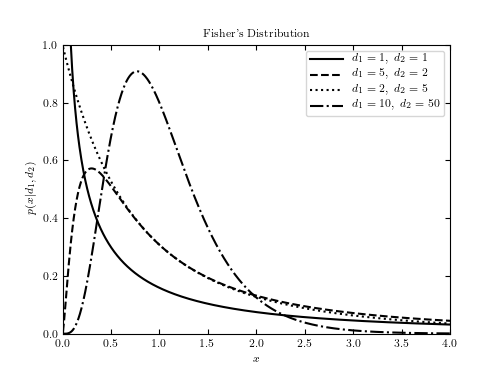
Example of Fisher’s F distribution
This shows an example of Fisher’s F distribution with various parameters. We’ll generate the distribution using:
Where … should be filled in with the desired distribution parameters Once we have defined the distribution parameters in this way, these distribution objects have many useful methods; for example:
- dist.pmf(x) computes the Probability Mass Function at values x in the case of discrete distributions
- dist.pdf(x) computes the Probability Density Function at values x in the case of continuous distributions
- dist.rvs(N) computes N random variables distributed according to the given distribution
Many further options exist; refer to the documentation of scipy.stats for more details.
Code output:
Python source code:
# Author: Jake VanderPlas # License: BSD # The figure produced by this code is published in the textbook # "Statistics, Data Mining, and Machine Learning in Astronomy" (2013) # For more information, see http://astroML.github.com # To report a bug or issue, use the following forum: # https://groups.google.com/forum/#!forum/astroml-general import numpy as np from scipy.stats import f as fisher_f from matplotlib import pyplot as plt #---------------------------------------------------------------------- # This function adjusts matplotlib settings for a uniform feel in the textbook. # Note that with usetex=True, fonts are rendered with LaTeX. This may # result in an error if LaTeX is not installed on your system. In that case, # you can set usetex to False. if "setup_text_plots" not in globals(): from astroML.plotting import setup_text_plots setup_text_plots(fontsize=8, usetex=True) #------------------------------------------------------------ # Define the distribution parameters to be plotted mu = 0 d1_values = [1, 5, 2, 10] d2_values = [1, 2, 5, 50] linestyles = ['-', '--', ':', '-.'] x = np.linspace(0, 5, 1001)[1:] fig, ax = plt.subplots(figsize=(5, 3.75)) for (d1, d2, ls) in zip(d1_values, d2_values, linestyles): dist = fisher_f(d1, d2, mu) plt.plot(x, dist.pdf(x), ls=ls, c='black', label=r'$d_1=%i,\ d_2=%i$' % (d1, d2)) plt.xlim(0, 4) plt.ylim(0.0, 1.0) plt.xlabel('$x$') plt.ylabel(r'$p(x|d_1, d_2)$') plt.title("Fisher's Distribution") plt.legend() plt.show()
scipy.stats.f#
As an instance of the rv_continuous class, f object inherits from it a collection of generic methods (see below for the full list), and completes them with details specific for this particular distribution.
The probability density function for f is:
for \(x > 0\) and parameters \(df_1, df_2 > 0\) .
f takes dfn and dfd as shape parameters.
The probability density above is defined in the “standardized” form. To shift and/or scale the distribution use the loc and scale parameters. Specifically, f.pdf(x, dfn, dfd, loc, scale) is identically equivalent to f.pdf(y, dfn, dfd) / scale with y = (x — loc) / scale . Note that shifting the location of a distribution does not make it a “noncentral” distribution; noncentral generalizations of some distributions are available in separate classes.
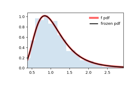
>>> import numpy as np >>> from scipy.stats import f >>> import matplotlib.pyplot as plt >>> fig, ax = plt.subplots(1, 1)
Calculate the first four moments:
>>> dfn, dfd = 29, 18 >>> mean, var, skew, kurt = f.stats(dfn, dfd, moments='mvsk')
Display the probability density function ( pdf ):
>>> x = np.linspace(f.ppf(0.01, dfn, dfd), . f.ppf(0.99, dfn, dfd), 100) >>> ax.plot(x, f.pdf(x, dfn, dfd), . 'r-', lw=5, alpha=0.6, label='f pdf')
Alternatively, the distribution object can be called (as a function) to fix the shape, location and scale parameters. This returns a “frozen” RV object holding the given parameters fixed.
Freeze the distribution and display the frozen pdf :
>>> rv = f(dfn, dfd) >>> ax.plot(x, rv.pdf(x), 'k-', lw=2, label='frozen pdf')
Check accuracy of cdf and ppf :
>>> vals = f.ppf([0.001, 0.5, 0.999], dfn, dfd) >>> np.allclose([0.001, 0.5, 0.999], f.cdf(vals, dfn, dfd)) True
And compare the histogram:
>>> ax.hist(r, density=True, bins='auto', histtype='stepfilled', alpha=0.2) >>> ax.set_xlim([x[0], x[-1]]) >>> ax.legend(loc='best', frameon=False) >>> plt.show()
rvs(dfn, dfd, loc=0, scale=1, size=1, random_state=None)
pdf(x, dfn, dfd, loc=0, scale=1)
Probability density function.
logpdf(x, dfn, dfd, loc=0, scale=1)
Log of the probability density function.
cdf(x, dfn, dfd, loc=0, scale=1)
Cumulative distribution function.
logcdf(x, dfn, dfd, loc=0, scale=1)
Log of the cumulative distribution function.
sf(x, dfn, dfd, loc=0, scale=1)
Survival function (also defined as 1 — cdf , but sf is sometimes more accurate).
logsf(x, dfn, dfd, loc=0, scale=1)
Log of the survival function.
ppf(q, dfn, dfd, loc=0, scale=1)
Percent point function (inverse of cdf — percentiles).
isf(q, dfn, dfd, loc=0, scale=1)
Inverse survival function (inverse of sf ).
moment(order, dfn, dfd, loc=0, scale=1)
Non-central moment of the specified order.
stats(dfn, dfd, loc=0, scale=1, moments=’mv’)
Mean(‘m’), variance(‘v’), skew(‘s’), and/or kurtosis(‘k’).
entropy(dfn, dfd, loc=0, scale=1)
(Differential) entropy of the RV.
Parameter estimates for generic data. See scipy.stats.rv_continuous.fit for detailed documentation of the keyword arguments.
expect(func, args=(dfn, dfd), loc=0, scale=1, lb=None, ub=None, conditional=False, **kwds)
Expected value of a function (of one argument) with respect to the distribution.
median(dfn, dfd, loc=0, scale=1)
Median of the distribution.
mean(dfn, dfd, loc=0, scale=1)
var(dfn, dfd, loc=0, scale=1)
Variance of the distribution.
std(dfn, dfd, loc=0, scale=1)
Standard deviation of the distribution.
interval(confidence, dfn, dfd, loc=0, scale=1)
Confidence interval with equal areas around the median.
scipy.stats.fisher_exact#
Perform a Fisher exact test on a 2×2 contingency table.
The null hypothesis is that the true odds ratio of the populations underlying the observations is one, and the observations were sampled from these populations under a condition: the marginals of the resulting table must equal those of the observed table. The statistic returned is the unconditional maximum likelihood estimate of the odds ratio, and the p-value is the probability under the null hypothesis of obtaining a table at least as extreme as the one that was actually observed. There are other possible choices of statistic and two-sided p-value definition associated with Fisher’s exact test; please see the Notes for more information.
Parameters : table array_like of ints
A 2×2 contingency table. Elements must be non-negative integers.
Defines the alternative hypothesis. The following options are available (default is ‘two-sided’):
- ‘two-sided’: the odds ratio of the underlying population is not one
- ‘less’: the odds ratio of the underlying population is less than one
- ‘greater’: the odds ratio of the underlying population is greater than one
See the Notes for more details.
Returns : res SignificanceResult
An object containing attributes:
This is the prior odds ratio, not a posterior estimate.
The probability under the null hypothesis of obtaining a table at least as extreme as the one that was actually observed.
Chi-square test of independence of variables in a contingency table. This can be used as an alternative to fisher_exact when the numbers in the table are large.
Compute the odds ratio (sample or conditional MLE) for a 2×2 contingency table.
Barnard’s exact test, which is a more powerful alternative than Fisher’s exact test for 2×2 contingency tables.
Boschloo’s exact test, which is a more powerful alternative than Fisher’s exact test for 2×2 contingency tables.
Null hypothesis and p-values
The null hypothesis is that the true odds ratio of the populations underlying the observations is one, and the observations were sampled at random from these populations under a condition: the marginals of the resulting table must equal those of the observed table. Equivalently, the null hypothesis is that the input table is from the hypergeometric distribution with parameters (as used in hypergeom ) M = a + b + c + d , n = a + b and N = a + c , where the input table is [[a, b], [c, d]] . This distribution has support max(0, N + n — M)