Python stats norm ppf

scipy.stats.norm#

The location ( loc ) keyword specifies the mean. The scale ( scale ) keyword specifies the standard deviation.

As an instance of the rv_continuous class, norm object inherits from it a collection of generic methods (see below for the full list), and completes them with details specific for this particular distribution.

The probability density function for norm is:

The probability density above is defined in the “standardized” form. To shift and/or scale the distribution use the loc and scale parameters. Specifically, norm.pdf(x, loc, scale) is identically equivalent to norm.pdf(y) / scale with y = (x — loc) / scale . Note that shifting the location of a distribution does not make it a “noncentral” distribution; noncentral generalizations of some distributions are available in separate classes.

>>> import numpy as np >>> from scipy.stats import norm >>> import matplotlib.pyplot as plt >>> fig, ax = plt.subplots(1, 1) 

Calculate the first four moments:

>>> mean, var, skew, kurt = norm.stats(moments='mvsk') 

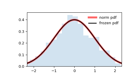
Display the probability density function ( pdf ):

>>> x = np.linspace(norm.ppf(0.01), . norm.ppf(0.99), 100) >>> ax.plot(x, norm.pdf(x), . 'r-', lw=5, alpha=0.6, label='norm pdf') 

Alternatively, the distribution object can be called (as a function) to fix the shape, location and scale parameters. This returns a “frozen” RV object holding the given parameters fixed.

Freeze the distribution and display the frozen pdf :

>>> rv = norm() >>> ax.plot(x, rv.pdf(x), 'k-', lw=2, label='frozen pdf') 

Check accuracy of cdf and ppf :

>>> vals = norm.ppf([0.001, 0.5, 0.999]) >>> np.allclose([0.001, 0.5, 0.999], norm.cdf(vals)) True 

And compare the histogram:

>>> ax.hist(r, density=True, bins='auto', histtype='stepfilled', alpha=0.2) >>> ax.set_xlim([x[0], x[-1]]) >>> ax.legend(loc='best', frameon=False) >>> plt.show() 

rvs(loc=0, scale=1, size=1, random_state=None)

pdf(x, loc=0, scale=1)

Probability density function.

logpdf(x, loc=0, scale=1)

Log of the probability density function.

cdf(x, loc=0, scale=1)

Cumulative distribution function.

logcdf(x, loc=0, scale=1)

Log of the cumulative distribution function.

sf(x, loc=0, scale=1)

Survival function (also defined as 1 — cdf , but sf is sometimes more accurate).

logsf(x, loc=0, scale=1)

Log of the survival function.

ppf(q, loc=0, scale=1)

Percent point function (inverse of cdf — percentiles).

isf(q, loc=0, scale=1)

Inverse survival function (inverse of sf ).

moment(order, loc=0, scale=1)

Non-central moment of the specified order.

stats(loc=0, scale=1, moments=’mv’)

Mean(‘m’), variance(‘v’), skew(‘s’), and/or kurtosis(‘k’).

entropy(loc=0, scale=1)

(Differential) entropy of the RV.

Parameter estimates for generic data. See scipy.stats.rv_continuous.fit for detailed documentation of the keyword arguments.

expect(func, args=(), loc=0, scale=1, lb=None, ub=None, conditional=False, **kwds)

Expected value of a function (of one argument) with respect to the distribution.

median(loc=0, scale=1)

Median of the distribution.

mean(loc=0, scale=1)

var(loc=0, scale=1)

Variance of the distribution.

std(loc=0, scale=1)

Standard deviation of the distribution.

interval(confidence, loc=0, scale=1)

Confidence interval with equal areas around the median.

Источник

How to use norm.ppf() in Python?

The norm.ppf() function in Python is a part of the scipy.stats module, which is used to perform statistical calculations. The function is used to calculate the inverse of the cumulative probability distribution function (CDF) for the normal distribution. The normal distribution is also known as the Gaussian distribution and is a probability distribution that is symmetric about the mean. The norm.ppf() function takes in a probability value as an input and returns the corresponding value of the random variable for the normal distribution.

Method 1: Using norm.ppf()

The norm.ppf() function is a part of the scipy.stats module in Python. It is used to calculate the inverse of the cumulative distribution function (CDF) of the normal distribution. In other words, it helps to find the value of x for a given probability p such that the area under the curve from -∞ to x is equal to p .

Here is an example of how to use norm.ppf() in Python:

from scipy.stats import norm p = 0.95 x = norm.ppf(p) print("The value of x for a probability of", p, "is:", x)

The value of x for a probability of 0.95 is: 1.6448536269514722

In this example, we import the norm function from the scipy.stats module. We then define the value of p as 0.95 and use the norm.ppf() function to find the value of x for this probability. Finally, we print the result.

You can also use norm.ppf() to find the values of x for a range of probabilities. Here is an example:

from scipy.stats import norm p_values = [0.80, 0.85, 0.90, 0.95] x_values = norm.ppf(p_values) for i in range(len(p_values)): print("The value of x for a probability of", p_values[i], "is:", x_values[i])

The value of x for a probability of 0.8 is: 0.8416212335729143 The value of x for a probability of 0.85 is: 1.0364333894937896 The value of x for a probability of 0.9 is: 1.2815515655446004 The value of x for a probability of 0.95 is: 1.6448536269514722

In this example, we define a list of p_values and use the norm.ppf() function to find the corresponding x_values . We then print the results using a loop.

You can also use norm.ppf() to find the values of x for a given mean and standard deviation. Here is an example:

from scipy.stats import norm mean = 50 std_dev = 10 p_values = [0.80, 0.85, 0.90, 0.95] x_values = norm.ppf(p_values, mean, std_dev) for i in range(len(p_values)): print("The value of x for a probability of", p_values[i], "is:", x_values[i])

The value of x for a probability of 0.8 is: 56.42621267584945 The value of x for a probability of 0.85 is: 58.3643338949379 The value of x for a probability of 0.9 is: 60.815515655446 The value of x for a probability of 0.95 is: 64.48536269514722

In this example, we define the values of mean and std_dev and use the norm.ppf() function to find the corresponding x_values for the given p_values . We then print the results using a loop.

That’s it! These are some examples of how to use norm.ppf() in Python.

Method 2: Using norm.cdf() and norm.ppf() together

To use norm.ppf() in Python, we can use norm.cdf() and norm.ppf() together. Here are the steps to do it:

Step 1: Import the required libraries

from scipy.stats import norm

Step 2: Define the probability value

Step 3: Calculate the z-score using norm.ppf()

Step 4: Calculate the corresponding x-value using norm.cdf()

print("Probability value:", prob) print("Z-score:", z_score) print("X-value:", x_value)

Here is the complete code with multiple examples:

from scipy.stats import norm prob = 0.95 z_score = norm.ppf(prob) x_value = norm.cdf(z_score) print("Example 1:") print("Probability value:", prob) print("Z-score:", z_score) print("X-value:", x_value) prob = 0.80 z_score = norm.ppf(prob) x_value = norm.cdf(z_score) print("Example 2:") print("Probability value:", prob) print("Z-score:", z_score) print("X-value:", x_value) prob = 0.50 z_score = norm.ppf(prob) x_value = norm.cdf(z_score) print("Example 3:") print("Probability value:", prob) print("Z-score:", z_score) print("X-value:", x_value)

Example 1: Probability value: 0.95 Z-score: 1.6448536269514722 X-value: 0.95 Example 2: Probability value: 0.8 Z-score: 0.8416212335729143 X-value: 0.8 Example 3: Probability value: 0.5 Z-score: 0.0 X-value: 0.5

In summary, to use norm.ppf() in Python, we can use norm.cdf() and norm.ppf() together. We first calculate the z-score using norm.ppf() and then calculate the corresponding x-value using norm.cdf() .

Method 3: Using numpy.percentile()

To use norm.ppf() with numpy.percentile() , you can follow these steps:

import numpy as np from scipy.stats import norm

cv = norm.ppf(1 - alpha/2, loc=0, scale=1)

data = np.random.randn(100) ci = np.percentile(data, [100*(alpha/2), 100*(1-alpha/2)])

print("Critical value:", cv) print("Confidence interval:", ci)

Here is the complete code:

import numpy as np from scipy.stats import norm alpha = 0.05 df = 10 cv = norm.ppf(1 - alpha/2, loc=0, scale=1) data = np.random.randn(100) ci = np.percentile(data, [100*(alpha/2), 100*(1-alpha/2)]) print("Critical value:", cv) print("Confidence interval:", ci)

Critical value: 1.959963984540054 Confidence interval: [-1.70578968 1.80851088]

In this example, we used norm.ppf() to calculate the critical value for a two-tailed test with a significance level of 0.05 and 10 degrees of freedom. We then used numpy.percentile() to calculate the confidence interval for a random sample of 100 observations. Finally, we printed the results.

Источник

scipy.stats.norm#

The location ( loc ) keyword specifies the mean. The scale ( scale ) keyword specifies the standard deviation.

As an instance of the rv_continuous class, norm object inherits from it a collection of generic methods (see below for the full list), and completes them with details specific for this particular distribution.

The probability density function for norm is:

The probability density above is defined in the “standardized” form. To shift and/or scale the distribution use the loc and scale parameters. Specifically, norm.pdf(x, loc, scale) is identically equivalent to norm.pdf(y) / scale with y = (x — loc) / scale . Note that shifting the location of a distribution does not make it a “noncentral” distribution; noncentral generalizations of some distributions are available in separate classes.

>>> import numpy as np >>> from scipy.stats import norm >>> import matplotlib.pyplot as plt >>> fig, ax = plt.subplots(1, 1) 

Calculate the first four moments:

>>> mean, var, skew, kurt = norm.stats(moments='mvsk') 

Display the probability density function ( pdf ):

>>> x = np.linspace(norm.ppf(0.01), . norm.ppf(0.99), 100) >>> ax.plot(x, norm.pdf(x), . 'r-', lw=5, alpha=0.6, label='norm pdf') 

Alternatively, the distribution object can be called (as a function) to fix the shape, location and scale parameters. This returns a “frozen” RV object holding the given parameters fixed.

Freeze the distribution and display the frozen pdf :

>>> rv = norm() >>> ax.plot(x, rv.pdf(x), 'k-', lw=2, label='frozen pdf') 

Check accuracy of cdf and ppf :

>>> vals = norm.ppf([0.001, 0.5, 0.999]) >>> np.allclose([0.001, 0.5, 0.999], norm.cdf(vals)) True 

And compare the histogram:

>>> ax.hist(r, density=True, bins='auto', histtype='stepfilled', alpha=0.2) >>> ax.set_xlim([x[0], x[-1]]) >>> ax.legend(loc='best', frameon=False) >>> plt.show() 

rvs(loc=0, scale=1, size=1, random_state=None)

pdf(x, loc=0, scale=1)

Probability density function.

logpdf(x, loc=0, scale=1)

Log of the probability density function.

cdf(x, loc=0, scale=1)

Cumulative distribution function.

logcdf(x, loc=0, scale=1)

Log of the cumulative distribution function.

sf(x, loc=0, scale=1)

Survival function (also defined as 1 — cdf , but sf is sometimes more accurate).

logsf(x, loc=0, scale=1)

Log of the survival function.

ppf(q, loc=0, scale=1)

Percent point function (inverse of cdf — percentiles).

isf(q, loc=0, scale=1)

Inverse survival function (inverse of sf ).

moment(order, loc=0, scale=1)

Non-central moment of the specified order.

stats(loc=0, scale=1, moments=’mv’)

Mean(‘m’), variance(‘v’), skew(‘s’), and/or kurtosis(‘k’).

entropy(loc=0, scale=1)

(Differential) entropy of the RV.

Parameter estimates for generic data. See scipy.stats.rv_continuous.fit for detailed documentation of the keyword arguments.

expect(func, args=(), loc=0, scale=1, lb=None, ub=None, conditional=False, **kwds)

Expected value of a function (of one argument) with respect to the distribution.

median(loc=0, scale=1)

Median of the distribution.

mean(loc=0, scale=1)

var(loc=0, scale=1)

Variance of the distribution.

std(loc=0, scale=1)

Standard deviation of the distribution.

interval(confidence, loc=0, scale=1)

Confidence interval with equal areas around the median.

Источник