Python ssa time series

Saved searches

Use saved searches to filter your results more quickly

You signed in with another tab or window. Reload to refresh your session. You signed out in another tab or window. Reload to refresh your session. You switched accounts on another tab or window. Reload to refresh your session.

Python implementation of Monte Carlo Singular Spectrum Analysis for univariate time series.

VSainteuf/mcssa

This commit does not belong to any branch on this repository, and may belong to a fork outside of the repository.

Name already in use

A tag already exists with the provided branch name. Many Git commands accept both tag and branch names, so creating this branch may cause unexpected behavior. Are you sure you want to create this branch?

Sign In Required

Please sign in to use Codespaces.

Launching GitHub Desktop

If nothing happens, download GitHub Desktop and try again.

Launching GitHub Desktop

If nothing happens, download GitHub Desktop and try again.

Launching Xcode

If nothing happens, download Xcode and try again.

Launching Visual Studio Code

Your codespace will open once ready.

There was a problem preparing your codespace, please try again.

Latest commit

Git stats

Files

Failed to load latest commit information.

README.md

Python module to compute univariate Monte Carlo Singular Spectrum Analysis on python3

Allen, Myles R., and Leonard A. Smith. «Monte Carlo SSA: Detecting Irregular Oscillations in the Presence of Colored Noise.» Journal of Climate 9, no. 12 (1996): 3373-404. http://www.jstor.org/stable/26201460.

Clone repo on your machine and cd into the parent folder. You can then locally install the package with:

Python3 with basic libraries (numpy, scipy, pandas and matplotlib)

The steps of the following example can be found in the main of mcssa.py

Take an example time series containing an oscillatory component and some random noise

import numpy as np import matplotlib.pyplot as plt from mcssa.mcssa import SSA,MCSSA T = 8 series = [np.sin(2 * np.pi / T * i) + np.random.rand() for i in range(100)]

Perform a Singular Spectrum Analysis of the series with a window length of M=20

ssa = SSA(series) ssa.run_ssa(20) ssa.plot(freq_rank=True)

The resulting plot gives an estimate of the spectrum of the series:

One can see a pair of EOFs with very high variance in the 0.125 cycles per time unit (cpu) range, corresponding to a 8 time unit period. The precise value of the dominant frequencies can be obtained with ssa.show_f() . The reconstruction of the time series corresponding to these EOFs can be obtained with:

RC=ssa.reconstruct([0,1]) RC.plot()

Now assume that the time series at study was given to us and that we have no a priori knowledge on it. We would like to know if the spectral peak at 0.125 cpu is containing signal or could have just been generated by random coloured noise.

In that aim we perform a Monte Carlo SSA, to determine the extent to which an AR(1) process could have obtained similar variance on the data’s EOFs. We use the same window lenght M=20 and set the simulation to 5000 realisations.

mcssa = MCSSA(series) mcssa.run_mcssa(20, n_suro=5000) mcssa.plot()

In the resulting spectrum the two supspected EOFs appear far above the 95% error bars, indicating that the power they contain in the data series is statistically significant. The precise significance can be obtained with mcssa.scores .

Once the presence of signal in these two EOFs has been proven, they can be set aside in a second test to check for other potential significant EOFs:

mcssa.run_mcssa(20, n_suro=5000,filtered_components=[0,1]) mcssa.plot()

No further signal is detected as the remaining EOFs’ variances lie within the error bars.

About

Python implementation of Monte Carlo Singular Spectrum Analysis for univariate time series.

Источник

Saved searches

Use saved searches to filter your results more quickly

You signed in with another tab or window. Reload to refresh your session. You signed out in another tab or window. Reload to refresh your session. You switched accounts on another tab or window. Reload to refresh your session.

Python Singular Spectrum Analysis using various embedding methods and SVD algorithms

GERUlab/vassal

This commit does not belong to any branch on this repository, and may belong to a fork outside of the repository.

Name already in use

A tag already exists with the provided branch name. Many Git commands accept both tag and branch names, so creating this branch may cause unexpected behavior. Are you sure you want to create this branch?

Sign In Required

Please sign in to use Codespaces.

Launching GitHub Desktop

If nothing happens, download GitHub Desktop and try again.

Launching GitHub Desktop

If nothing happens, download GitHub Desktop and try again.

Launching Xcode

If nothing happens, download Xcode and try again.

Launching Visual Studio Code

Your codespace will open once ready.

There was a problem preparing your codespace, please try again.

Latest commit

Git stats

Files

Failed to load latest commit information.

README.md

VASSAL: VArious Singular Spectrum AnaLysis with python

• Compatibility with python 3
• Computing the weighted correlation matrix is too long for large time series
• Reconstructing series is too long for long time series
• Make ‘paired’ plot able to plot any pair, not just consecutive one
• Implement Toeplitz SSA
• Add a decimal in the characteristic contribution
• Add a method for change point analysis that uses Singular Spectrum Transansformation (SST)

What is Singular Spectrum Analysis?

Singular Spectrum Analysis (SSA) is a non-parametric and model free method for time series decomposition, reconstruction (and foracasting). The general walktrhough of SSA consists in (1) embedding the time series into a trajectory matrix of lagged vectors, (2) decomposing the trajectory matrix using singular value decomposition (SVD), (3) grouping the resulting components based on similarities between their singular values or eigenvectors to reconstruct interpretable components of the original time series. The later is usually supervised.

The main hypothesis behind SSA is separability of the components.

Potential application of SSA

• Smoothing, filtering, noise reduction
• Structured components extraction (ie. trend or seasonality)
• Filling missing values
• Forecasting
• Nonlinear time series analysis

Different variants of SSA could be declined based either on the embedding method, the decomposition method or the dimensional nature of the dataset of interest.

• Basic SSA: The basic 1d SSA algorithm also known as the Broomhead-King variant of SSA (or BK-SSA). The time series is embedded in a Hankel matrix.
• Toeplitz SSA: The Toeplitz variant of SSA also known as Vautard-Ghil variant of SSA (or VG-SSA). The time series is embedded in a Toeplitz matrix. Toeplitz SSA should be used when time series is known to be stationary.
• SSA-ICA: ICA refers to Independent Component Analysis (ICA) and replace SVD. This variants helps to separate components in case of weak separability. As a less stable procedure than SVD, SSA-ICA is best used in a two stages procedure, a first separation is done using a basic SVD method, then remaining mixed-up components are decomposed using SSA-ICA.

Some other variants are not 1-dimensional such as: Multichannel SSA (multiple time series), 2d-SSA (arrays and images), nd-SSA (nd arrays).

Comparison with rSSA package:

rSSA package uses either ‘nutrlan’, ‘propack’, ‘full svd’ with the dgesdd routine and ‘eigen’ as full SVD via eigendecompsition of the cross-product matrix

Here is a little longer answer to your question on comparing ARPACK with TRLan. TRLan (and nuTRLan) implements a restarted version of Lanczos algorithm, just like ARPACK implements a restarted version of Arnoldi algorithm. In this regard, the user has control over the memory usage by controlling the maximum basis size. Another similarity is that both can keep an arbitrary number of basis vectors when restarting — this is the key advantage of these methods over earlier restarted versions. On symmetric (or Hermitian) problems, when the basis vectors corresponding to the same Ritz values are saved during restarting, TRLan and ARPACK are theoretically equivalent. One difference is that TRLan uses Ritz vectors while ARPACK uses the vectors produced by the implicit QR procedure. This makes TRLan a little easier to understand and implement. This difference is mainly useful for software implementors — it is of no consequence to the end users. What do have some consequence are the following. TRLan can take advantage of the symmetry in the original problem as Ichi has pointed out. TRLan and especially nuTRLan use more advanced strategies to decide what Ritz values to save during restarting. These strategies have been demonstrated to be very effective. In general, the restarted version of Lanczos would need more matrix-vector multiplications than the un-restarted version. In cases where the un-restarted Lanczos can be used, TRLan was shown to use nearly the same number of matrix-vector multiplications. On more difficult eigenvalue problems, TRLan usually performed better because of the new restarting strategies.

References for sklearn TruncatedSVD:

• Finding structure with randomness: Stochastic algorithms for constructing approximate matrix decompositions Halko, et al., 2009 http://arxiv.org/abs/arXiv:0909.4061
• A randomized algorithm for the decomposition of matrices Per-Gunnar Martinsson, Vladimir Rokhlin and Mark Tygert
• An implementation of a randomized algorithm for principal component analysis A. Szlam et al. 2014

SVD algorithms in python scientific librairies

The decomposition is performed using LAPACK, with option ´full_matrices´,

The decompotion is performed usin LAPACK, with option ´full_matrices´, additionnaly the user can choose a lapack_driver.

Compute the largest k singular values/vectors for a sparse matrix. This is a naive implementation using ARPACK as an eigensolver on A.H * A or A * A.H, depending on which one is more efficient.

This estimator supports two algorithms: a fast randomized SVD solver, and a “naive” algorithm that uses ARPACK as an eigensolver on (X * X.T) or (X.T * X), whichever is more efficient.

Both nplapack and splapack use the LAPACK algorithm for full svd decomposition but the scipy implementation allows more flexibility. Hence it is kept. The same goes with sparpack and skarpack , as skarpack is just a wrapper to sparpack with fewer arguments allowed. To my knowledge, skrandom has no equivalent.

Are kept: splapack , sparpack and skrandom .

[1] Singular Spectrum Analysis for Time Series | Nina Golyandina | Springer. Accessed November 19, 2017. //www.springer.com/gp/book/9783642349126.

About

Python Singular Spectrum Analysis using various embedding methods and SVD algorithms

Источник

Singular Spectrum Analysis¶

Signals such as time series can be seen as a sum of different signals such as trends and noise. Decomposing time series into several time series can be useful in order to keep the most important information. One decomposition algorithm is Singular Spectrum Analysis. This example illustrates the decomposition of a time series into several subseries using this algorithm and visualizes the different subseries extracted. It is implemented as pyts.decomposition.SingularSpectrumAnalysis .

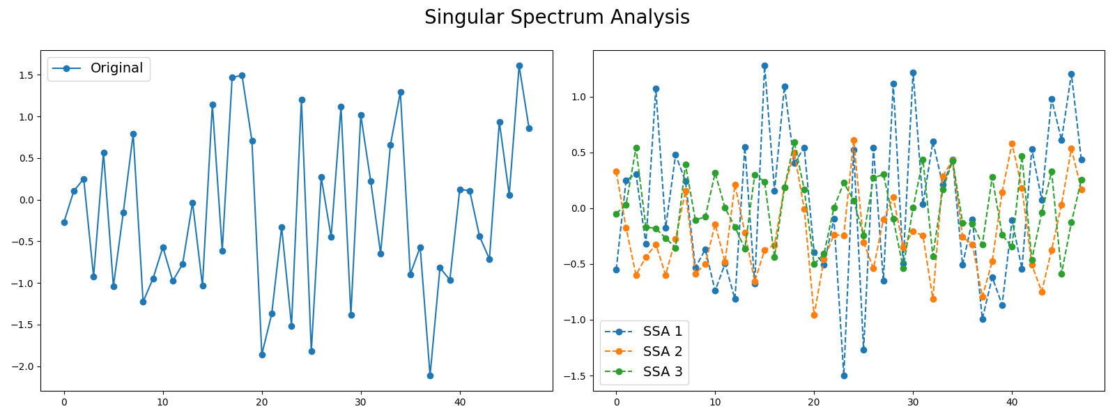
# Author: Johann Faouzi # License: BSD-3-Clause import numpy as np import matplotlib.pyplot as plt from pyts.decomposition import SingularSpectrumAnalysis # Parameters n_samples, n_timestamps = 100, 48 # Toy dataset rng = np.random.RandomState(41) X = rng.randn(n_samples, n_timestamps) # We decompose the time series into three subseries window_size = 15 groups = [np.arange(i, i + 5) for i in range(0, 11, 5)] # Singular Spectrum Analysis ssa = SingularSpectrumAnalysis(window_size=15, groups=groups) X_ssa = ssa.fit_transform(X) # Show the results for the first time series and its subseries plt.figure(figsize=(16, 6)) ax1 = plt.subplot(121) ax1.plot(X[0], 'o-', label='Original') ax1.legend(loc='best', fontsize=14) ax2 = plt.subplot(122) for i in range(len(groups)): ax2.plot(X_ssa[0, i], 'o--', label='SSA '.format(i + 1)) ax2.legend(loc='best', fontsize=14) plt.suptitle('Singular Spectrum Analysis', fontsize=20) plt.tight_layout() plt.subplots_adjust(top=0.88) plt.show() # The first subseries consists of the trend of the original time series. # The second and third subseries consist of noise. 

Total running time of the script: ( 0 minutes 3.361 seconds)

Источник