Python pandas dataframe statistics

Как рассчитать сводную статистику для Pandas DataFrame

Вы можете использовать следующие методы для расчета сводной статистики для переменных в pandas DataFrame:

Метод 1: вычислить сводную статистику для всех числовых переменных

Метод 2: вычислить сводную статистику для всех строковых переменных

Метод 3: вычислить сводную статистику, сгруппированную по переменной

df.groupby('group_column').mean() df.groupby('group_column'). median () df.groupby('group_column'). max () . 

В следующих примерах показано, как использовать каждый метод на практике со следующими пандами DataFrame:

import pandas as pd import numpy as np #create DataFrame df = pd.DataFrame() #view DataFrame print(df) team points assists rebounds 0 A 18 5.0 11.0 1 A 22 NaN 8.0 2 A 19 7.0 10.0 3 A 14 9.0 6.0 4 B 14 12.0 6.0 5 B 11 9.0 5.0 6 B 20 9.0 9.0 7 B 28 4.0 NaN 8 B 30 5.0 6.0 

Пример 1. Расчет сводной статистики для всех числовых переменных

В следующем коде показано, как рассчитать сводную статистику для каждой числовой переменной в DataFrame:

df.describe () points assists rebounds count 9.000000 8.000000 8.000000 mean 19.555556 7.500000 7.625000 std 6.366143 2.725541 2.199838 min 11.000000 4.000000 5.000000 25% 14.000000 5.000000 6.000000 50% 19.000000 8.000000 7.000000 75% 22.000000 9.000000 9.250000 max 30.000000 12.000000 11.000000 

Мы можем видеть следующую сводную статистику для каждой из трех числовых переменных:

• count: количество ненулевых значений
• среднее : среднее значение
• std : стандартное отклонение
• мин: минимальное значение
• 25% : значение на 25-м процентиле.
• 50% : значение на 50-м процентиле (также медиана)
• 75% : значение на 75-м процентиле.
• макс : максимальное значение

Пример 2. Расчет сводной статистики для всех строковых переменных

В следующем коде показано, как рассчитать сводную статистику для каждой строковой переменной в DataFrame:

df.describe (include='object') team count 9 unique 2 top B freq 5 

Мы можем увидеть следующую сводную статистику для одной строковой переменной в нашем DataFrame:

• count : количество ненулевых значений
• unique : Количество уникальных значений
• top: наиболее часто встречающееся значение
• freq : количество наиболее часто встречающихся значений

Пример 3. Вычисление сводной статистики, сгруппированной по переменной

В следующем коде показано, как вычислить среднее значение для всех числовых переменных, сгруппированных по переменной команды :

df.groupby('team').mean() points assists rebounds team A 18.25 7.0 8.75 B 20.60 7.8 6.50 

В выходных данных отображается среднее значение переменных очков , передач и подборов , сгруппированных по переменной команды .

Обратите внимание, что мы можем использовать аналогичный синтаксис для вычисления другой сводной статистики, такой как медиана:

df.groupby('team'). median () points assists rebounds team A 18.5 7.0 9.0 B 20.0 9.0 6.0 

В выходных данных отображается среднее значение переменных очков , передач и подборов , сгруппированных по переменной команды .

Примечание.Вы можете найти полную документацию для функции описания в pandas здесь .

Дополнительные ресурсы

В следующих руководствах объясняется, как выполнять другие распространенные задачи в pandas:

Источник

pandas.DataFrame.describe#

Descriptive statistics include those that summarize the central tendency, dispersion and shape of a dataset’s distribution, excluding NaN values.

Analyzes both numeric and object series, as well as DataFrame column sets of mixed data types. The output will vary depending on what is provided. Refer to the notes below for more detail.

Parameters percentiles list-like of numbers, optional

The percentiles to include in the output. All should fall between 0 and 1. The default is [.25, .5, .75] , which returns the 25th, 50th, and 75th percentiles.

include ‘all’, list-like of dtypes or None (default), optional

A white list of data types to include in the result. Ignored for Series . Here are the options:

• ‘all’ : All columns of the input will be included in the output.
• A list-like of dtypes : Limits the results to the provided data types. To limit the result to numeric types submit numpy.number . To limit it instead to object columns submit the numpy.object data type. Strings can also be used in the style of select_dtypes (e.g. df.describe(include=[‘O’]) ). To select pandas categorical columns, use ‘category’
• None (default) : The result will include all numeric columns.

A black list of data types to omit from the result. Ignored for Series . Here are the options:

• A list-like of dtypes : Excludes the provided data types from the result. To exclude numeric types submit numpy.number . To exclude object columns submit the data type numpy.object . Strings can also be used in the style of select_dtypes (e.g. df.describe(exclude=[‘O’]) ). To exclude pandas categorical columns, use ‘category’
• None (default) : The result will exclude nothing.

Summary statistics of the Series or Dataframe provided.

Count number of non-NA/null observations.

Maximum of the values in the object.

Minimum of the values in the object.

Standard deviation of the observations.

Subset of a DataFrame including/excluding columns based on their dtype.

For numeric data, the result’s index will include count , mean , std , min , max as well as lower, 50 and upper percentiles. By default the lower percentile is 25 and the upper percentile is 75 . The 50 percentile is the same as the median.

For object data (e.g. strings or timestamps), the result’s index will include count , unique , top , and freq . The top is the most common value. The freq is the most common value’s frequency. Timestamps also include the first and last items.

If multiple object values have the highest count, then the count and top results will be arbitrarily chosen from among those with the highest count.

For mixed data types provided via a DataFrame , the default is to return only an analysis of numeric columns. If the dataframe consists only of object and categorical data without any numeric columns, the default is to return an analysis of both the object and categorical columns. If include=’all’ is provided as an option, the result will include a union of attributes of each type.

The include and exclude parameters can be used to limit which columns in a DataFrame are analyzed for the output. The parameters are ignored when analyzing a Series .

Describing a numeric Series .

>>> s = pd.Series([1, 2, 3]) >>> s.describe() count 3.0 mean 2.0 std 1.0 min 1.0 25% 1.5 50% 2.0 75% 2.5 max 3.0 dtype: float64 

Describing a categorical Series .

>>> s = pd.Series(['a', 'a', 'b', 'c']) >>> s.describe() count 4 unique 3 top a freq 2 dtype: object 

Describing a timestamp Series .

>>> s = pd.Series([ . np.datetime64("2000-01-01"), . np.datetime64("2010-01-01"), . np.datetime64("2010-01-01") . ]) >>> s.describe() count 3 mean 2006-09-01 08:00:00 min 2000-01-01 00:00:00 25% 2004-12-31 12:00:00 50% 2010-01-01 00:00:00 75% 2010-01-01 00:00:00 max 2010-01-01 00:00:00 dtype: object 

Describing a DataFrame . By default only numeric fields are returned.

>>> df = pd.DataFrame('categorical': pd.Categorical(['d','e','f']), . 'numeric': [1, 2, 3], . 'object': ['a', 'b', 'c'] . >) >>> df.describe() numeric count 3.0 mean 2.0 std 1.0 min 1.0 25% 1.5 50% 2.0 75% 2.5 max 3.0 

Describing all columns of a DataFrame regardless of data type.

>>> df.describe(include='all') categorical numeric object count 3 3.0 3 unique 3 NaN 3 top f NaN a freq 1 NaN 1 mean NaN 2.0 NaN std NaN 1.0 NaN min NaN 1.0 NaN 25% NaN 1.5 NaN 50% NaN 2.0 NaN 75% NaN 2.5 NaN max NaN 3.0 NaN 

Describing a column from a DataFrame by accessing it as an attribute.

>>> df.numeric.describe() count 3.0 mean 2.0 std 1.0 min 1.0 25% 1.5 50% 2.0 75% 2.5 max 3.0 Name: numeric, dtype: float64 

Including only numeric columns in a DataFrame description.

>>> df.describe(include=[np.number]) numeric count 3.0 mean 2.0 std 1.0 min 1.0 25% 1.5 50% 2.0 75% 2.5 max 3.0 

Including only string columns in a DataFrame description.

>>> df.describe(include=[object]) object count 3 unique 3 top a freq 1 

Including only categorical columns from a DataFrame description.

>>> df.describe(include=['category']) categorical count 3 unique 3 top d freq 1 

Excluding numeric columns from a DataFrame description.

>>> df.describe(exclude=[np.number]) categorical object count 3 3 unique 3 3 top f a freq 1 1 

Excluding object columns from a DataFrame description.

>>> df.describe(exclude=[object]) categorical numeric count 3 3.0 unique 3 NaN top f NaN freq 1 NaN mean NaN 2.0 std NaN 1.0 min NaN 1.0 25% NaN 1.5 50% NaN 2.0 75% NaN 2.5 max NaN 3.0 

Источник

Pandas Describe: Descriptive Statistics on Your Dataframe

In this tutorial, you’ll learn how to use the Pandas describe method, which is used to computer summary descriptive statistics for your Pandas Dataframe. By the end of reading this tutorial, you’ll have learned how to use the Pandas .describe() method to generate summary statistics and how to modify it using its different parameters, to make sure you get the results you’re hoping for.

Being able to understand your data using high-level summary statistics is an important first step in your exploratory data analysis (EDA). It’s a helpful first step in your data science work, that opens up your work to statistics you may want to explore further.

The Pandas .describe() method provides you with generalized descriptive statistics that summarize the central tendency of your data, the dispersion, and the shape of the dataset’s distribution. It also provides helpful information on missing NaN data.

The Quick Answer: Pandas describe Provides Helpful Summary Statistics

Loading a Sample Pandas Dataframe

If you want to follow along with the tutorial on the Pandas describe method, feel free to copy the code below. The code will generate a dataframe based on the Seaborn library (which I cover off in great detail here). The library provides a number of datasets to guide you through different scenarios. These datasets are accessible via the load_dataset() function.

If you don’t have Seaborn installed, you can install it using either pip or conda. To install it with pip, simply write pip install seaborn into your terminal.

Let’s load a sample dataframe to follow along with:

# Loading a sample Pandas dataframe from seaborn import load_dataset df = load_dataset('penguins') print(df.head()) # Returns: species island bill_length_mm bill_depth_mm flipper_length_mm body_mass_g sex 0 Adelie Torgersen 39.1 18.7 181.0 3750.0 Male 1 Adelie Torgersen 39.5 17.4 186.0 3800.0 Female 2 Adelie Torgersen 40.3 18.0 195.0 3250.0 Female 3 Adelie Torgersen NaN NaN NaN NaN NaN 4 Adelie Torgersen 36.7 19.3 193.0 3450.0 Female

We can see, that by printing out the first five records of our dataframe using the Pandas .head() method, that our dataframe has seven columns. Some of these columns are numeric, while others contain string values. However, beyond that, we can’t see much else about the data in the dataframe, such as the distribution of the data itself.

This is where the Pandas describe method comes into play! In the next section, you’ll learn how to generate some summary statistics using the Pandas describe method.

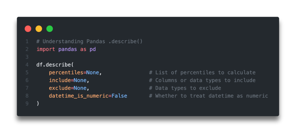
Understanding the Pandas describe Method

The Pandas describe method is a helpful dataframe method that returns descriptive and summary statistics. The method will return items such:

• The number of items
• Measures of dispersion
• Measures of central tendency
• Percentiles of data
• Maximum and minumum values

Let’s break down the various arguments available in the Pandas .describe() method:

Источник