Python matplotlib data file

Plot data from excel file in matplotlib Python

This tutorial is the one in which you will learn a basic method required for data science. That skill is to plot the data from an excel file in matplotlib in Python. Here you will learn to plot data as a graph in the excel file using matplotlib and pandas in Python.

How to plot data from excel file using matplotlib?

Before we plot the data from excel file in matplotlib, first we have to take care of a few things.

• You must have these packages installed in your IDE:- matplotlib, pandas, xlrd.
• Save an Excel file on your computer in any easily accessible location.
• If you are doing this coding in command prompt or shell, then make sure your directories and packages are correctly managed.
• For the sake of simplicity, we will be doing this using any IDE available.

Step 1: Import the pandas and matplotlib libraries.

import pandas as pd import matplotlib.pyplot as plt

Step 2 : read the excel file using pd.read_excel( ‘ file location ‘) .

var = pd.read_excel('C:\\user\\name\\documents\\officefiles.xlsx') var.head()

To let the interpreter know that the following \ is to be ignored as the escape sequence, we use two \.
the “var” is the data frame name. To display the first five rows in pandas we use the data frame .head() function.

If you have multiple sheets, then to focus on one sheet we will mention that after reading the file location.

var = pd.read_excel('C:\\user\\name\\documents\\officefiles.xlsx','Sheet1') var.head()

Step 3: To select a given column or row.
Here you can select a specific range of rows and columns that you want to be displayed. Just by making a new list and mentioning the columns name.

varNew = var[['column1','column2','column3']] varNew.head()

To select data to be displayed after specific rows, use ‘skip rows’ attribute.

var = pd.read_excel('C:\\user\\name\\documents\\officefiles.xlsx', skiprows=6)

step 4: To plot the graph of the selected files column.
to plot the data just add plt.plot(varNew[‘column name’]) . Use plt.show() to plot the graph.

import matplotlib.pyplot as plt import pandas as pd var= pd.read_excel('C:\\Users\\name\\Documents\\officefiles.xlsx') plt.plot(var['column name']) var.head() plt.show()

You will get the Graph of the data as the output.

You may also love to learn:

Источник

Data Visualizing from CSV Format to Chart using Python

In this article, we will download a data set from an online resource and create a working visualization of that data. As we have discussed in the previous article, the internet is being bombarded by lots of data each second. An incredible amount and variety of data can be found online. The ability to analyze data allows you to discover the patterns and connections.

We will access and visualize the data store in CSV format. We will use Python’s CSV module to process weather data. We will analyze the high and low temperatures over the period in two different locations. Then we will use matplotlib to generate a chart.

By the end of this article, you’ll be able to work with different datasets and build complex visualizations. It is essential to be able to access and visualize online data which contains a wide variety of real-world datasets.

The CSV File Format

CSV stands for Comma Separated Values. As the name suggests, it is a kind of file in which values are separated by commas.

It is one of the simpler ways to store the data in a textual format as a series of comma separated values. The resulting file is called a CSV file.

For example, below given is a line of weather data on which we are going to work in this article.

2014-1-6,62,43,52,18,7,-1,56,33,9,30.3,30.2,. . ., 195

This is the weather data. We will start with a small dataset. It is CSV formatted data Stika, Alaska. You can download datasets from https://www.wunderground.com. This is how your CSV file of data will look like:

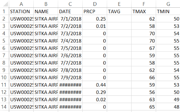
The first line is called the header.

Parsing the CSV File Headers

We can easily parse the values and extract the required information using the Python’s csv module. Let’s start by analyzing the first line of the file which contains the headers used for data.

1. Create a python file name weather_data.py

2. Write the following statement to import the CSV module:

3. Download the data file from here.

4. Open the file using Python’s open function and print the headers:

filename = ‘sitka_weather_07-2018_simple.csv’ with open(filename) as f: reader = csv.reader(f) #line 1 header_row = next(reader) #line 2 print(header_row) #line 3

After importing the CSV module, we store the name of the file in the variable filename. We then open the file using the open function and store the result file object in f.

Next, on line 1, we have called the reader function of the CSV module and passed the file object f to it as an argument. This function creates a reader object associated with that file.

The CSV module contains a next() function which returns the next line in the file. next() function accepts a reader object as an argument. So, it returns the next line of the file with which reader object is associated. We only need to call the next() function once to get the first line of the file which contains header normally. So, the header is stored in the variable header_row . The next line, just prints the header row.

Here is the output of the above code snippet:

[‘STATION’, ‘NAME’, ‘DATE’, ‘AWND’, ‘PGTM’, ‘PRCP’, ‘SNWD’, ‘TAVG’, ‘TMAX’, ‘TMIN’, ‘WDF2’, ‘WDF5’, ‘WSF2’, ‘WSF5’, ‘WT01’, ‘WT02’, ‘WT04’, ‘WT05’, ‘WT08’]

reader processes the first line of comma-separated values and stores each as an item in the list. For example, TMAX denotes maximum temperature for that day.

Printing the Headers with their positions

We usually print header with their position in the list, to make it easier to understand the file header data.

import csv filename = 'sitka_weather_2018_full.csv' with open(filename) as f: reader = csv.reader(f) header_row = next(reader) for index,column_header in enumerate(header_row): print(index, column_header)

Output:

We have used the enumerate() function on the list to get the index of each item in the list and as well the value. NOTE: We have removed the print(header_row) line to get a more detailed version of data.

Here we can see that the date and respective max temperature are stored in column 2 and 8 respectively. Let’s extract these.

Extracting and Reading Data

Now that we know which columns of data we need, let’s read in some of that data. First, we’ll read in the high temperature for each day:

highs = [] for row in reader: highs.append(row[8]) #appending high temperatures print(highs)

We make an empty list named highs. Then, we iterate through each row in the reader and keep appending the high temperature which is available on index 8 to the list. The reader object continues from where it left in the CSV file and automatically returns a new line on its current position. Then we print the list. It looks like below:

[’48’, ’48’, ’46’, ’42’, ’46’, ’44’, ’39’, ’36’, ’34’, ’28’, ’34’, ’41’, ’53’, ’63’, ’60’, ’54’, ’47’, ’46’, ’42’, ’45’, ’43’, ’41’, ’41’, ’40’, … , ]

As we can see that list returned is in the form of strings. Now, we convert these strings to number using int() so that they can be read by matplotlib.

for row in reader: if row[8] == ‘’: continue # There are some empty strings which can’t be converted to int high = int(row[8]) #Convert to int highs.append(high) #appending high temperatures

Now our data is ready to for plotting.

[48, 48, 46, 42, 46, 44, 39, 36, 34, 28, 34, 41, 53, 63, 60, 54, 47, 46, 42, 45, 43, 41, 41, 40, 40, 41, 39, 40, 40, 39, 36, 35, 35, 34, 42, 41, 39, 42, 39, 37, 37, 40, 43, 41, 40, 38, 36, 37, 39, 39, 38, 41, 42, 41, 39, 38, 42, 39, 40,. . ., ]

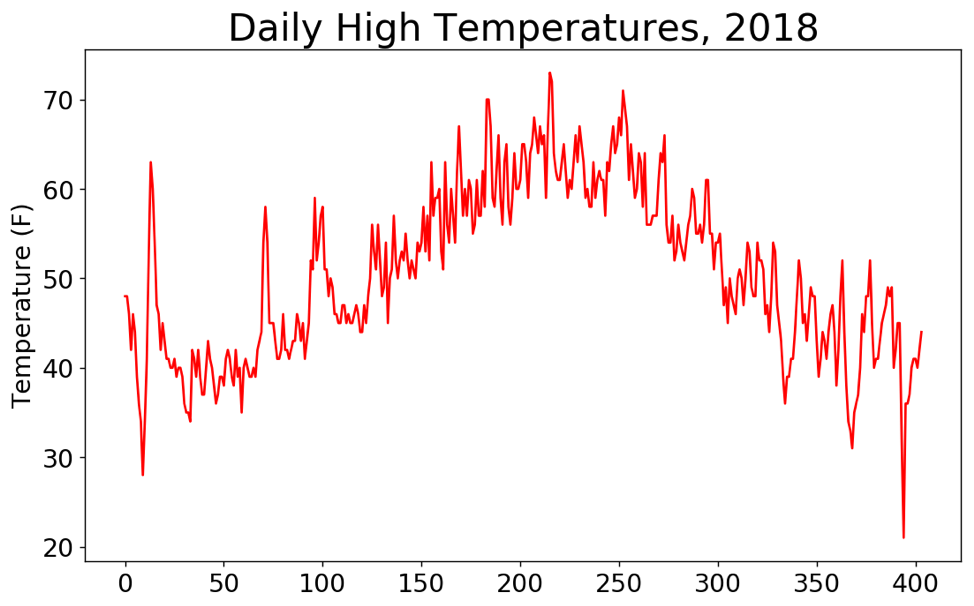
Plotting Data in Temperature Chart using Matplotlib

To visualize the temperature data, we will first create a plot of daily high temperatures using matplotlib.

import csv from matplotlib import pyplot as plt filename = 'sitka_weather_2018_full.csv' with open(filename) as f: reader = csv.reader(f) header_row = next(reader) highs = [] for row in reader: if row[8]=='': continue high = int(row[8],10) highs.append(high) #appending high temperatures #Plot Data fig = plt.figure(dpi = 128, figsize = (10,6)) plt.plot(highs, c = 'red') #Line 1 #Format Plot plt.title("Daily High Temperatures, 2018", fontsize = 24) plt.xlabel('',fontsize = 16) plt.ylabel("Temperature (F)", fontsize = 16) plt.tick_params(axis = 'both', which = 'major' , labelsize = 16) plt.show()

Running the Above Code, you’ll get this.

Thank you for reading. I hope It will be helpful. Comment If you find any difficulty. I’ll love to solve your problem.

Here’re some more Articles, you might be interested:

Источник

Plotting data from a file¶

Plotting data from a file is actually a two-step process.

pyplot.plotfile tried to do both at once. But each of the steps has so many possible variations and parameters that it does not make sense to squeeze both into a single function. Therefore, pyplot.plotfile has been deprecated.

The recommended way of plotting data from a file is therefore to use dedicated functions such as numpy.loadtxt or pandas.read_csv to read the data. These are more powerful and faster. Then plot the obtained data using matplotlib.

Note that pandas.DataFrame.plot is a convenient wrapper around Matplotlib to create simple plots.

import matplotlib.pyplot as plt import matplotlib.cbook as cbook import numpy as np import pandas as pd 

Using pandas¶

Subsequent are a few examples of how to replace plotfile with pandas . All examples need the the pandas.read_csv call first. Note that you can use the filename directly as a parameter:

The following slightly more involved pandas.read_csv call is only to make automatic rendering of the example work:

fname = cbook.get_sample_data('msft.csv', asfileobj=False) with cbook.get_sample_data('msft.csv') as file: msft = pd.read_csv(file) 

When working with dates, additionally call pandas.plotting.register_matplotlib_converters and use the parse_dates argument of pandas.read_csv :

pd.plotting.register_matplotlib_converters()

with cbook.get_sample_data(‘msft.csv’) as file: msft = pd.read_csv(file, parse_dates=[‘Date’])

Use indices¶

# Deprecated: plt.plotfile(fname, (0, 5, 6)) # Use instead: msft.plot(0, [5, 6], subplots=True) 

Use names¶

# Deprecated: plt.plotfile(fname, ('date', 'volume', 'adj_close')) # Use instead: msft.plot("Date", ["Volume", "Adj. Close*"], subplots=True) 

Use semilogy for volume¶

# Deprecated: plt.plotfile(fname, ('date', 'volume', 'adj_close'), plotfuncs='volume': 'semilogy'>) # Use instead: fig, axs = plt.subplots(2, sharex=True) msft.plot("Date", "Volume", ax=axs[0], logy=True) msft.plot("Date", "Adj. Close*", ax=axs[1]) 

Use semilogy for volume (by index)¶

# Deprecated: plt.plotfile(fname, (0, 5, 6), plotfuncs=5: 'semilogy'>) # Use instead: fig, axs = plt.subplots(2, sharex=True) msft.plot(0, 5, ax=axs[0], logy=True) msft.plot(0, 6, ax=axs[1]) 

Single subplot¶

# Deprecated: plt.plotfile(fname, ('date', 'open', 'high', 'low', 'close'), subplots=False) # Use instead: msft.plot("Date", ["Open", "High", "Low", "Close"]) 

Use bar for volume¶

# Deprecated: plt.plotfile(fname, (0, 5, 6), plotfuncs=5: "bar">) # Use instead: fig, axs = plt.subplots(2, sharex=True) axs[0].bar(msft.iloc[:, 0], msft.iloc[:, 5]) axs[1].plot(msft.iloc[:, 0], msft.iloc[:, 6]) fig.autofmt_xdate() 

Using numpy¶

fname2 = cbook.get_sample_data('data_x_x2_x3.csv', asfileobj=False) with cbook.get_sample_data('data_x_x2_x3.csv') as file: array = np.loadtxt(file) 

Labeling, if no names in csv-file¶

# Deprecated: plt.plotfile(fname2, cols=(0, 1, 2), delimiter=' ', names=['$x$', '$f(x)=x^2$', '$f(x)=x^3$']) # Use instead: fig, axs = plt.subplots(2, sharex=True) axs[0].plot(array[:, 0], array[:, 1]) axs[0].set(ylabel='$f(x)=x^2$') axs[1].plot(array[:, 0], array[:, 2]) axs[1].set(xlabel='$x$', ylabel='$f(x)=x^3$') 

More than one file per figure¶

# For simplicity of the example we reuse the same file. # In general they will be different. fname3 = fname2 # Depreacted: plt.plotfile(fname2, cols=(0, 1), delimiter=' ') plt.plotfile(fname3, cols=(0, 2), delimiter=' ', newfig=False) # use current figure plt.xlabel(r'$x$') plt.ylabel(r'$f(x) = x^2, x^3$') # Use instead: fig, ax = plt.subplots() ax.plot(array[:, 0], array[:, 1]) ax.plot(array[:, 0], array[:, 2]) ax.set(xlabel='$x$', ylabel='$f(x)=x^3$') plt.show() 

Keywords: matplotlib code example, codex, python plot, pyplot Gallery generated by Sphinx-Gallery

© Copyright 2002 — 2012 John Hunter, Darren Dale, Eric Firing, Michael Droettboom and the Matplotlib development team; 2012 — 2018 The Matplotlib development team.
Last updated on Jun 17, 2020. Created using Sphinx 3.1.1. Doc version v3.2.2-2-g137edd56a.

Источник