Python matplotlib bar stacked

Matplotlib — Stacked Bar Plots

After learning about simple bar plots in the previous tutorial, it’s time to take a look at stacked bar plots. Stacked bar plots provide more detail information about every individual bar. Let’s dive in!

Matplotlib Series Overview

Stacked Bar Plots

In the simple bar plot tutorial, you used the number of tutorials we have published on Future Studio each year. But there was no differentiation between public and 🌟 premium tutorials. With stacked bar plots, we can still show the number of tutorials are published each year on Future Studio, but now also showing how many of them are public or premium.

Here’s the data you can use in this tutorial:

import matplotlib.pyplot as plt year = [2014, 2015, 2016, 2017, 2018, 2019] tutorial_public = [39, 117, 98, 54, 28, 15] tutorial_premium = [ 0, 0, 13, 56, 39, 14] 

As you can see from the number, we shifted from mainly public tutorials in 2014 to 2016 to a more balanced publishing in the last few years.

So let’s take a look at how you can create stacked bar plots. In the last tutorial, you learned that you can combine different styles of bar plots by calling the bar() method multiple times. You create stacked bar plots the same way, the first bar() call will be the amount of public tutorials with the standard options, but need to tweak the second method call to plot the premium tutorials.

When you call bar() a second time to create new bar plots above the already existing ones, you specify that they don’t start at 0, but at the value of the public tutorials of that year with the bottom parameter. To make the plot prettier, we change the color as well with the color parameter.

# the first call is as usual plt.bar(year, tutorial_public, color="#6c3376") # the second one is special to create stacked bar plots plt.bar(year, tutorial_premium, bottom=tutorial_public, color="#f3e151") plt.xlabel('Year') plt.ylabel('Number of futurestud.io Tutorials') plt.show()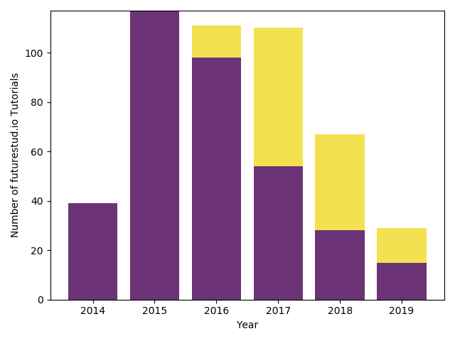 

With only a handful of lines of code, you created your first nice stacked bar plot:

As you probably already realized, you have fine control over which bar will be on top. Let’s switch them.

Stack Bar Plot (Switched)

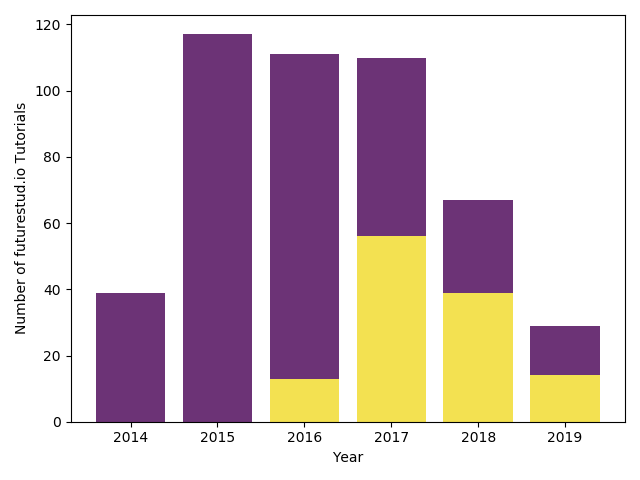
In recent years, the premium tutorials have been the base of Future Studio. Maybe they should be at the bottom while public tutorials are just a bonus on top?

You can simply create such a plot by changing which data you pass to each call.

year = [2014, 2015, 2016, 2017, 2018, 2019] tutorial_public = [39, 117, 98, 54, 28, 15] tutorial_premium = [0, 0, 13, 56, 39, 14] plt.bar(year, tutorial_premium, color="#f3e151") plt.bar(year, tutorial_public, bottom=tutorial_premium, color="#6c3376") plt.xlabel('Year') plt.ylabel('Number of futurestud.io Tutorials') plt.show() 

This results in a similar plot, just with the public and premium tutorials switched:

Horizontal Stacked Bar Plots

You still have the same customization options you have learned in the previous tutorials (for example, edgecolor ). In this last example, you will create a horizontal stacked bar plot.

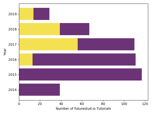
If you want to create horizontal instead of the default vertical plots, you need to call barh() instead of bar() . For stacked bar plots, you need to make one further change. The bottom parameter changes to the left parameter, which makes sense if you visualize the plot, but something to pay attention to when changing to a horizontal plot.

year = [2014, 2015, 2016, 2017, 2018, 2019] tutorial_public = [39, 117, 98, 54, 28, 15] tutorial_premium = [0, 0, 13, 56, 39, 14] plt.barh(year, tutorial_premium, color="#f3e151") # careful: notice "bottom" parameter became "left" plt.barh(year, tutorial_public, left=tutorial_premium, color="#6c3376") # we also need to switch the labels plt.xlabel('Number of futurestud.io Tutorials') plt.ylabel('Year') plt.show() 

Don’t forget to also switch the labels!

This will result in a pretty horizontal stacked bar plot:

Summary

In this tutorial, you have learned the basics of creating stacked bar plots. Pay attention to passing the correct values to the bottom or left parameters to create correct plots!

All code is also available for easy copy & paste on a GitHub repository.

Do you have questions or feedback where this series should go? Let us know on Twitter @futurestud_io or leave a comment below.

Enjoy plotting & make it rock!

Mentioned Resources

Get Notified on New Future Studio
Content and Platform Updates

Get your weekly push notification about new and trending
Future Studio content and recent platform enhancements

Источник

Как создать гистограммы с накоплением в Matplotlib (с примерами)

Столбчатая диаграмма с накоплением — это тип диаграммы, в которой столбцы используются для отображения частоты различных категорий.

Мы можем создать этот тип диаграммы в Matplotlib, используя функцию matplotlib.pyplot.bar() .

В этом руководстве показано, как использовать эту функцию на практике.

Создайте базовую линейчатую диаграмму с накоплением

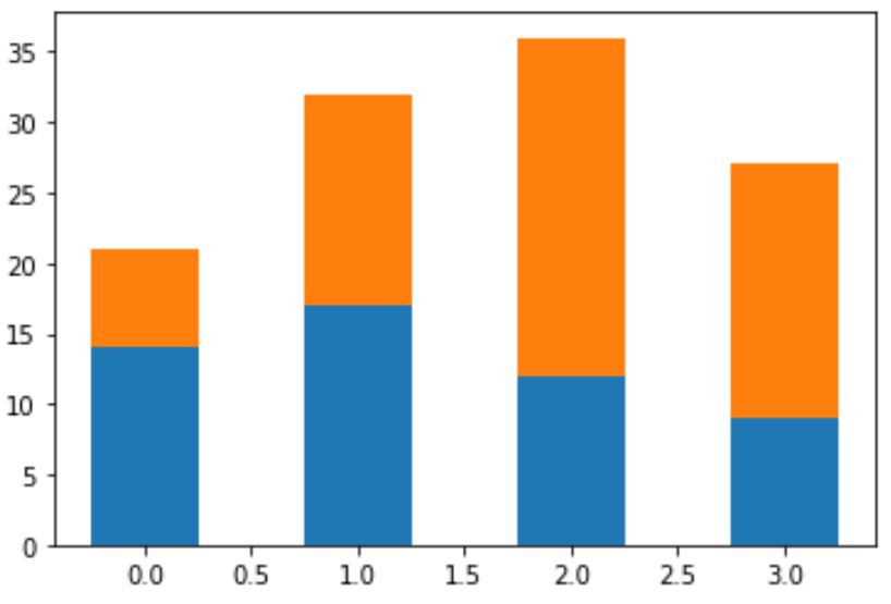
В следующем коде показано, как создать линейчатую диаграмму с накоплением для отображения общего объема продаж двух продуктов за четыре разных квартала продаж:

import numpy as np import matplotlib.pyplot as plt #create data quarter = ['Q1', 'Q2', 'Q3', 'Q4'] product_A = [14, 17, 12, 9] product_B = [7, 15, 24, 18] #define chart parameters N = 4 barWidth = .5 xloc = np.arange (N) #display stacked bar chart p1 = plt.bar (xloc, product_A, width=barWidth) p2 = plt.bar (xloc, product_B, bottom=product_A, width=barWidth) plt.show() 

Добавьте заголовок, метки и легенду

Мы также можем добавить заголовок, метки, деления и легенду, чтобы диаграмму было легче читать:

import numpy as np import matplotlib.pyplot as plt #create data for two teams quarter = ['Q1', 'Q2', 'Q3', 'Q4'] product_A = [14, 17, 12, 9] product_B = [7, 15, 24, 18] #define chart parameters N = 4 barWidth = .5 xloc = np.arange (N) #create stacked bar chart p1 = plt.bar (xloc, product_A, width=barWidth) p2 = plt.bar (xloc, product_B, bottom=product_A, width=barWidth) #add labels, title, tick marks, and legend plt.ylabel('Sales') plt.xlabel('Quarter') plt.title('Sales by Product & Quarter') plt.xticks (xloc,('Q1', 'Q2', 'Q3', 'Q4')) plt.yticks (np.arange (0, 41, 5)) plt.legend((p1[0], p2[0]),('A', 'B')) #display chart plt.show()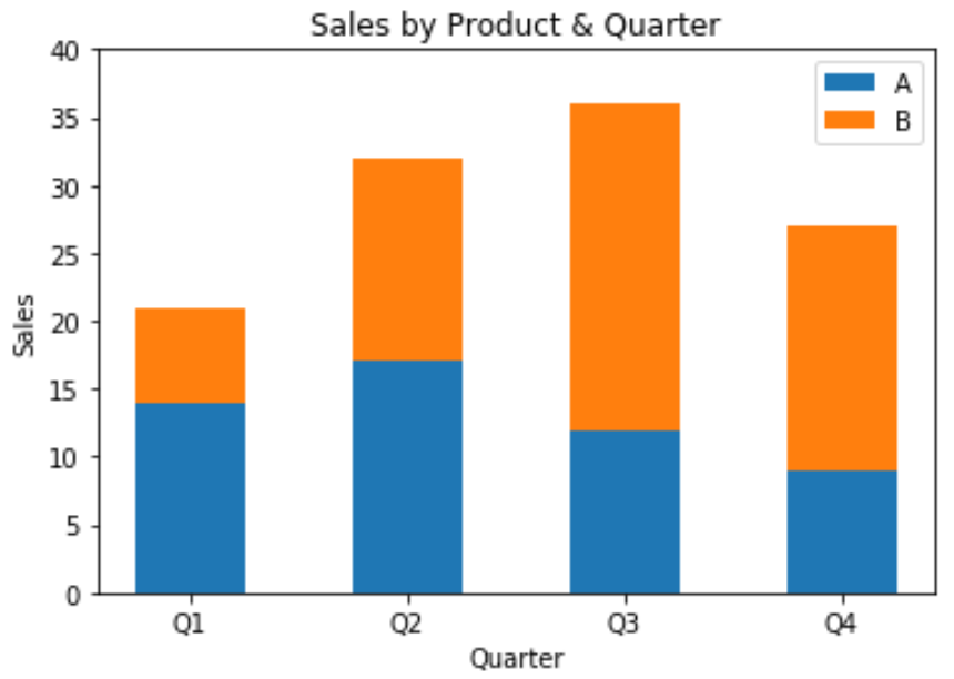 

Настройка цветов диаграммы

Наконец, мы можем настроить цвета, используемые в диаграмме, с помощью аргумента colors() в plt.bar() :

import numpy as np import matplotlib.pyplot as plt #create data for two teams quarter = ['Q1', 'Q2', 'Q3', 'Q4'] product_A = [14, 17, 12, 9] product_B = [7, 15, 24, 18] #define chart parameters N = 4 barWidth = .5 xloc = np.arange (N) #create stacked bar chart p1 = plt.bar (xloc, product_A, width=barWidth, color='springgreen') p2 = plt.bar (xloc, product_B, bottom=product_A, width=barWidth, color='coral') #add labels, title, tick marks, and legend plt.ylabel('Sales') plt.xlabel('Quarter') plt.title('Sales by Product & Quarter') plt.xticks (xloc,('Q1', 'Q2', 'Q3', 'Q4')) plt.yticks (np.arange (0, 41, 5)) plt.legend((p1[0], p2[0]),('A', 'B')) #display chart plt.show()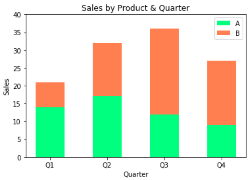 

Вы можете найти полный список доступных цветов в документации Matplotlib.

Дополнительные ресурсы

В следующих руководствах объясняется, как выполнять другие распространенные задачи в Matplotlib:

Источник

Stacked Bar Charts with Labels in Matplotlib

This post will go through a few examples of creating stacked bar charts using Matplotlib. We’ll look at some styling tweaks (like choosing custom colors) as well as go through how to add labels to the bars, both the totals and sub-totals for each bar.

And be sure to check out our related post on creating stacked bar charts using several python libraries beyond Matplotlib, like Seaborn and Altair.

Simple Stacked Bar Chart

The general idea for creating stacked bar charts in Matplotlib is that you’ll plot one set of bars (the bottom), and then plot another set of bars on top, offset by the height of the previous bars, so the bottom of the second set starts at the top of the first set. Sound confusing? It’s really not, so let’s get into it.

Let’s first get some data to work with.

import seaborn as sns tips = sns.load_dataset('tips') # Let's massage the data a bit to be aggregated by day of week, with # columns for each gender. We could leave it in long format as well ( # with gender as values in a single column). agg_tips = tips.groupby(['day', 'sex'])['tip'].sum().unstack().fillna(0) agg_tips 

Now let’s create our first chart. We want to know the total amount tipped by day of week, split out by gender.

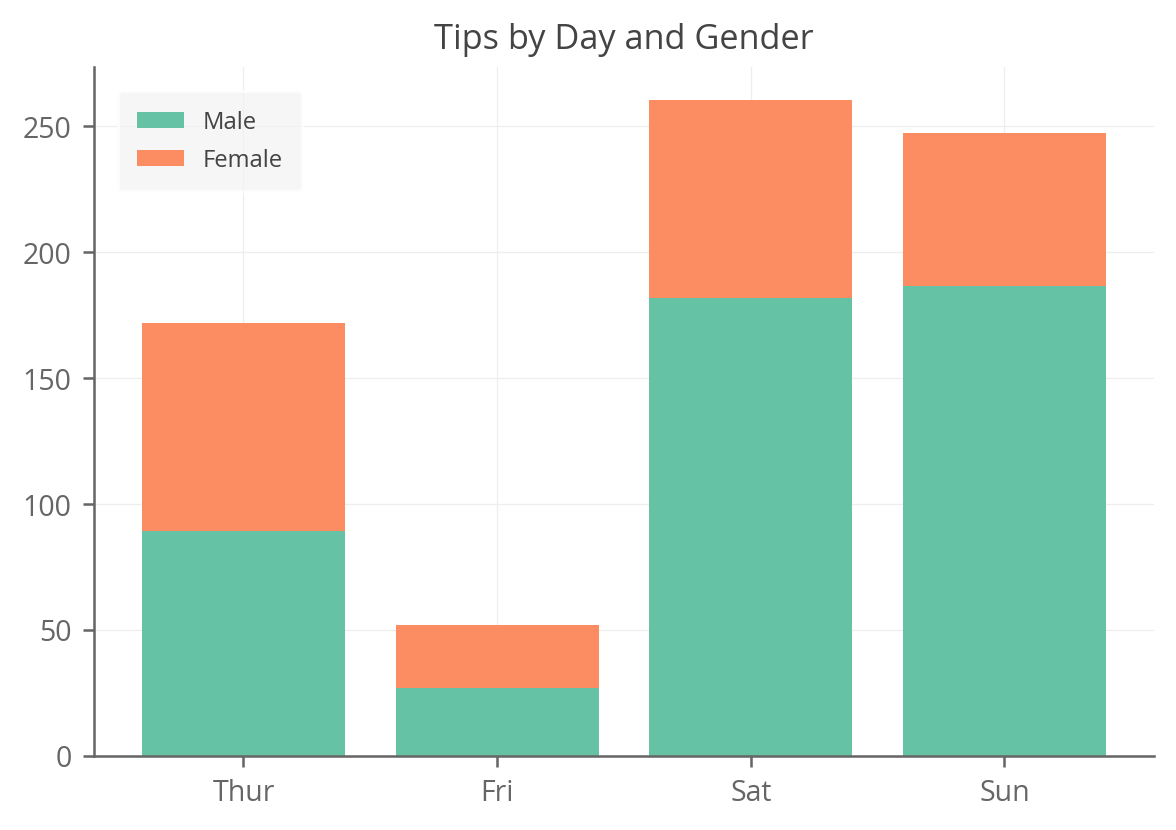
from matplotlib import pyplot as plt fig, ax = plt.subplots() # First plot the 'Male' bars for every day. ax.bar(agg_tips.index, agg_tips['Male'], label='Male') # Then plot the 'Female' bars on top, starting at the top of the 'Male' # bars. ax.bar(agg_tips.index, agg_tips['Female'], bottom=agg_tips['Male'], label='Female') ax.set_title('Tips by Day and Gender') ax.legend() 

As you can see, it’s pretty simple. We first plot tips that males gave and then plot tips that females gave, but give an additional bottom argument to tell Matplotlib where to start the bars (which happens to be the values of the previous bars; in this case male tips).

The above code generates this lovely plot:

Customizing the Stacked Bar Chart

The problem with the above code is that it starts to get very verbose, and quite repetitive, if we have more than a few layers in our stacked bars. So let’s make it a bit more DRY.

import numpy as np from matplotlib import pyplot as plt fig, ax = plt.subplots() # Initialize the bottom at zero for the first set of bars. bottom = np.zeros(len(agg_tips)) # Plot each layer of the bar, adding each bar to the "bottom" so # the next bar starts higher. for i, col in enumerate(agg_tips.columns): ax.bar(agg_tips.index, agg_tips[col], bottom=bottom, label=col) bottom += np.array(agg_tips[col]) ax.set_title('Tips by Day and Gender') ax.legend() 

This gives the exact same output as above, but is much nicer because we can apply it to any stacked bar need now, and it can handle as many layers as you need.

It’s also pretty flexible; for example, if we want to use custom colors we can easily do that:

fig, ax = plt.subplots() colors = ['#24b1d1', '#ae24d1'] bottom = np.zeros(len(agg_tips)) for i, col in enumerate(agg_tips.columns): ax.bar(agg_tips.index, agg_tips[col], bottom=bottom, label=col, color=colors[i]) bottom += np.array(agg_tips[col]) ax.set_title('Tips by Day and Gender') ax.legend() 

Adding Labels to the Bars

It’s often nice to add value labels to the bars in a bar chart. With a stacked bar chart, it’s a bit trickier, because you could add a total label or a label for each sub-bar within the stack. We’ll show you how to do both.

Adding a Total Label

We’ll do the same thing as above, but add a step where we compute the totals for each day of the week and then use ax.text() to add those above each bar.

fig, ax = plt.subplots() colors = ['#24b1d1', '#ae24d1'] bottom = np.zeros(len(agg_tips)) for i, col in enumerate(agg_tips.columns): ax.bar( agg_tips.index, agg_tips[col], bottom=bottom, label=col, color=colors[i]) bottom += np.array(agg_tips[col]) # Sum up the rows of our data to get the total value of each bar. totals = agg_tips.sum(axis=1) # Set an offset that is used to bump the label up a bit above the bar. y_offset = 4 # Add labels to each bar. for i, total in enumerate(totals): ax.text(totals.index[i], total + y_offset, round(total), ha='center', weight='bold') ax.set_title('Tips by Day and Gender') ax.legend() 

Adding both Sub-Bar and Total Labels

Now let’s do the same thing again, but this time, add annotations for each sub-bar in the stack. The method here is a bit different; we can actually get the patches or bars that we’ve already plotted, read their values, and then add those values as text annotations at the right location.

fig, ax = plt.subplots() colors = ['#24b1d1', '#ae24d1'] bottom = np.zeros(len(agg_tips)) for i, col in enumerate(agg_tips.columns): ax.bar( agg_tips.index, agg_tips[col], bottom=bottom, label=col, color=colors[i]) bottom += np.array(agg_tips[col]) totals = agg_tips.sum(axis=1) y_offset = 4 for i, total in enumerate(totals): ax.text(totals.index[i], total + y_offset, round(total), ha='center', weight='bold') # Let's put the annotations inside the bars themselves by using a # negative offset. y_offset = -15 # For each patch (basically each rectangle within the bar), add a label. for bar in ax.patches: ax.text( # Put the text in the middle of each bar. get_x returns the start # so we add half the width to get to the middle. bar.get_x() + bar.get_width() / 2, # Vertically, add the height of the bar to the start of the bar, # along with the offset. bar.get_height() + bar.get_y() + y_offset, # This is actual value we'll show. round(bar.get_height()), # Center the labels and style them a bit. ha='center', color='w', weight='bold', size=8 ) ax.set_title('Tips by Day and Gender') ax.legend()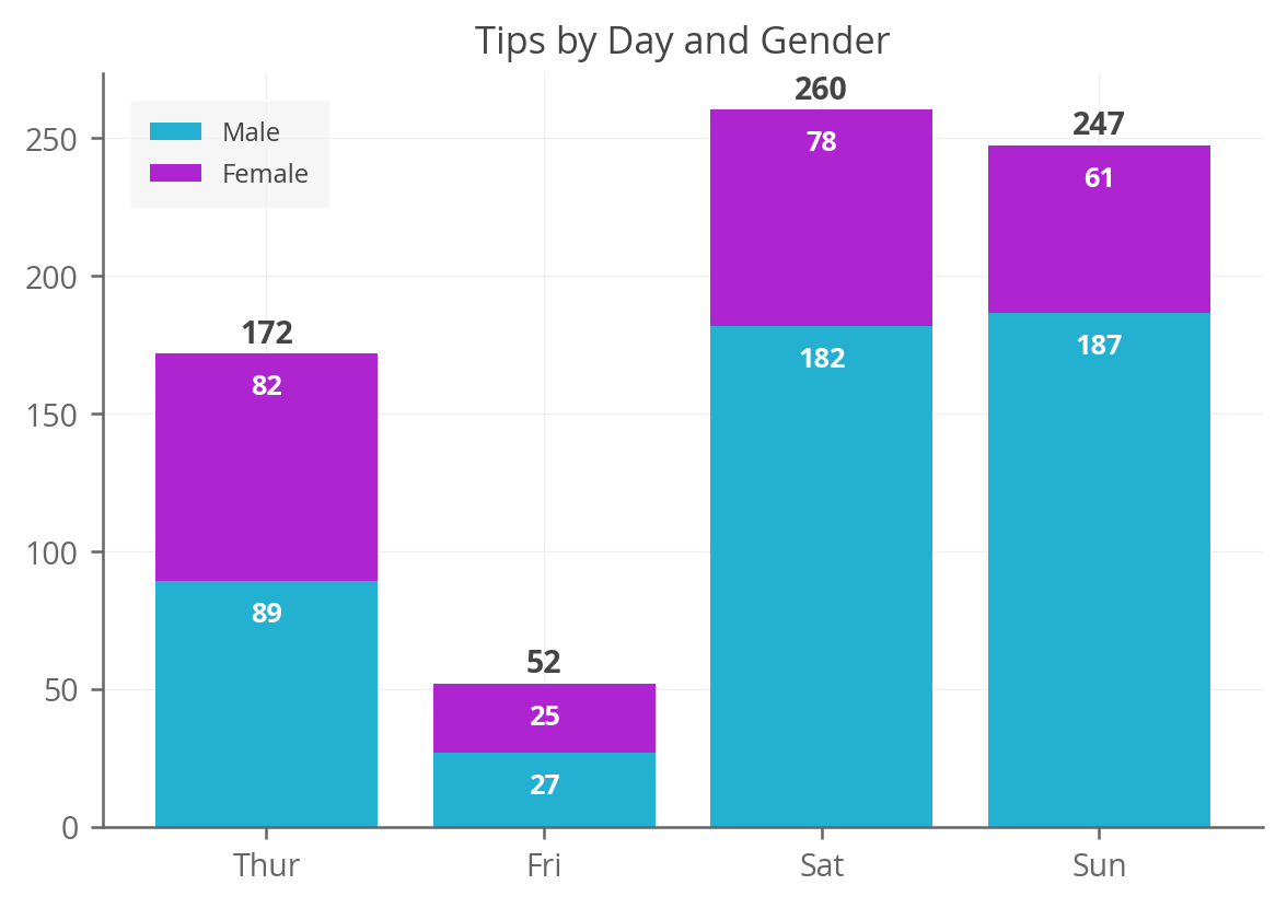 

Looks good. Thanks for reading and hopefully this helps get you on your way in creating annotated stacked bar charts in Matplotlib.

Источник