Python image histogram matching

Histogram Matching

How to generate a histogram for an image, how to equalize the histogram, and finally how to modify your image histogram to be similar to another histogram.

The code is available here on Github.

Please clap if you like the post.

What is an image histogram?

Before start defining the histogram, for simplicity, we use grayscales images. Then later I explain the process for the color images as well.

The image histogram indicates the intensity distribution of an image. In other words, the image histogram shows the number of pixels in an image having a specific intensity value. As an example, assume a normal image with pixel intensities varies from 0 to 255. In order to generate its histogram we only need to count the number of pixels having intensity value 0, then 1 and continue to the 255. In Fig.1, we have a sample 5*5 image with pixel diversities from 0 to 4. In the first step for generating the histogram, we create the Histogram Table, by counting the number of each pixel intensities. Then we can easily generate the histogram by creating a bar chart based on the histogram table.

How to generate an image histogram?

In python, we can use the following two functions to create and then display the histogram of an image.

In order to calculate the equalized histogram in python, I have created the following codes:

Enhancing images using equalized histogram

As mentioned, we can modify the contrast level of an image using its equalized histogram. As shown in Code.2, line #12, for each pixel in an input image, we can use its equalized value. The results might be better than the original image, but it is not guaranteed. In Fig.5, we depict the modified version of the 3 images. As shown, modifying the images using their equalized histogram results in images with a higher level of contrast. This feature can be useful in many computer vision tasks.

What is the histogram matching?

Assume we have two images and each has its specific histogram. So we want to answer this question before going further, is it possible to modify one image based on the contrast of another one? And the answer is YES. In fact, this is the definition of the histogram matching. In other words, given images A, and B, it is possible to modify the contrast level of A according to B.

Histogram matching is useful when we want to unify the contrast level of a group of images. In fact, Histogram equalization is also can be taken as histogram matching, since we modify the histogram of an input image to be similar to the normal distribution.

In order to match the histogram of images A and B, we need to first equalize the histogram of both images. Then, we need to map each pixel of A to B using the equalized histograms. Then we modify each pixel of A based on B.

Let’s clarify the above paragraph using the following example, in Fig.6.

In Fig.6, we have image A as the input image and Image B as the target image. We want to modify the histogram of A, based on the distribution of B. In the first step, we calculate both histogram and the equalized histogram of both A, and B. Then we need to map each pixel of A, based on the value of its equalized histogram to the value of B. So, for example for pixels with the intensity level of 0 in A, the corresponding value of A equalized histogram is 4. Now, we take a look at the B equalized histogram and find the intensity value corresponding to 4, which is 0. So we map the 0 intensity from A to 0 from B. We continue for all intensity values of A. If there is no map from the equalized histogram of A to B, we just need to pick the nearest value.

I have implemented the above process in Python as well

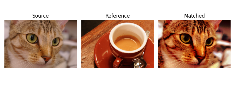
Fig.7 shown an example of histogram matching. As you see, while the leftmost image is a bright image, the center image can be considered a better image in terms of the contrast level. So, we decided to modify the leftmost using the contract of the center image. The result, which is the rightmost image has been improved.

Conclusion

In this article, I explained histogram matching which is a useful method while we cope with the images. I first started by explaining how to generate an image histogram. Then, how to equalize the generated histogram, and finally how to modify a picture based on the contrast level of another picture, called histogram matching. The code with the explanation is also available on Github.

The code is available here on Github.

Please clap if you like the post.

Источник

Histogram matching#

This example demonstrates the feature of histogram matching. It manipulates the pixels of an input image so that its histogram matches the histogram of the reference image. If the images have multiple channels, the matching is done independently for each channel, as long as the number of channels is equal in the input image and the reference.

Histogram matching can be used as a lightweight normalisation for image processing, such as feature matching, especially in circumstances where the images have been taken from different sources or in different conditions (i.e. lighting).

import matplotlib.pyplot as plt from skimage import data from skimage import exposure from skimage.exposure import match_histograms reference = data.coffee() image = data.chelsea() matched = match_histograms(image, reference, channel_axis=-1) fig, (ax1, ax2, ax3) = plt.subplots(nrows=1, ncols=3, figsize=(8, 3), sharex=True, sharey=True) for aa in (ax1, ax2, ax3): aa.set_axis_off() ax1.imshow(image) ax1.set_title('Source') ax2.imshow(reference) ax2.set_title('Reference') ax3.imshow(matched) ax3.set_title('Matched') plt.tight_layout() plt.show() 

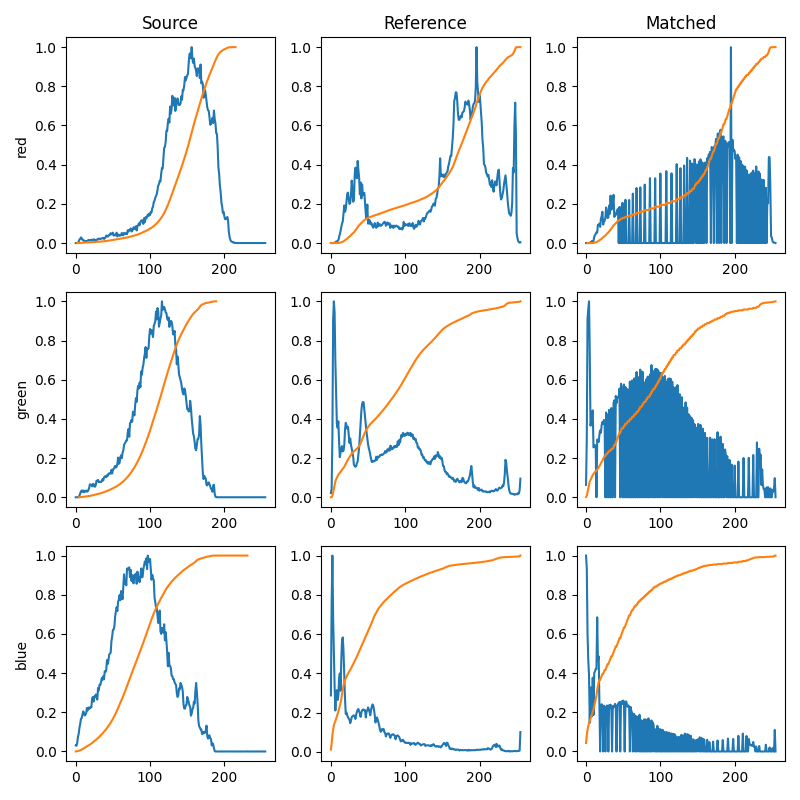
To illustrate the effect of the histogram matching, we plot for each RGB channel, the histogram and the cumulative histogram. Clearly, the matched image has the same cumulative histogram as the reference image for each channel.

fig, axes = plt.subplots(nrows=3, ncols=3, figsize=(8, 8)) for i, img in enumerate((image, reference, matched)): for c, c_color in enumerate(('red', 'green', 'blue')): img_hist, bins = exposure.histogram(img[. , c], source_range='dtype') axes[c, i].plot(bins, img_hist / img_hist.max()) img_cdf, bins = exposure.cumulative_distribution(img[. , c]) axes[c, i].plot(bins, img_cdf) axes[c, 0].set_ylabel(c_color) axes[0, 0].set_title('Source') axes[0, 1].set_title('Reference') axes[0, 2].set_title('Matched') plt.tight_layout() plt.show() 

Total running time of the script: ( 0 minutes 1.384 seconds)

Источник

Histogram Matching (Specification)

In the previous blog, we discussed Histogram Equalization that tries to produce an output image that has a uniform histogram. This approach is good but for some cases, this does not work well. One such case is when we have skewed image histogram i.e. large concentration of pixels at either end of greyscale.

One reasonable approach is to manually specify the transformation function that preserves the general shape of the original histogram but has a smoother transition of intensity levels in the skewed areas.

So, in this blog, we will learn how to transform an image so that its histogram matches a specified histogram. Also known as histogram matching or histogram Specification.

Histogram Equalization is a special case of histogram matching where the specified histogram is uniformly distributed.

First let’s understand the main idea behind histogram matching.

We will first equalize both original and specified histogram using the Histogram Equalization method. As we know that the transformation function is invertible, so by inverting we can get the mapping from original to specified histogram. The whole operation is shown in the below image

For example, suppose the pixel value 10 in the original image gets mapped to 20 in the equalized image. Then we will see what value in Specified image gets mapped to 20 in the equalized image and let’s say that this value is 28. So, we can say that 10 in the original image gets mapped to 28 in the specified image.

Most of you might be thinking why both original and specified histogram on equalization converges to same uniform histogram.

This is true only if we assume continuous intensity values. But in reality, the intensity values are discrete thus both original and specified histograms may not map to the same histogram on equalization. That’s why Histogram matching is not able to perfectly match the specified histogram.

Let’s take an example where we want to match the original image with the specified image, both histograms are shown below.

Here, I am taking the original image from the histogram equalization blog. All the steps of equalization are explained in this blog. Here, I will only show the final table

Original Image Histogram Equalization

Specified Image Histogram Equalization

After equalizing both the images, we need to perform a mapping from original to equalized to the specified image. For that, we need only the round columns of the original and specified image as shown below.

Pick one by one the values from the round column of the original image, find it in the round column of the specified image and note down the index. For example for 3 in the round original, we have 3 in the round specified column (with index 1) so we map it to 1.

If the value doesn’t exist then find the index of its nearest one. For example for 0 in round original, 1 is the nearest in round specified column (with index 0) so we map it to 0.

If multiple nearest values exist then pick the one which is greater than the value. For example for 2 in the round original, there are 2 closest values in round specified i.e. 1 and 3 so we pick 3 (with index 1) so we map it to 1.

After obtaining the Map column, replace the values in the original image with the map values. This is the final result.

The matched histogram(shown on left) approximately matches with the specified histogram(shown on right) as shown below

Now, let’s see how to perform Histogram matching using OpenCV-Python

Источник