Python augmented dickey fuller test

statsmodels.tsa.stattools.adfuller¶

The Augmented Dickey-Fuller test can be used to test for a unit root in a univariate process in the presence of serial correlation.

Parameters : ¶ x array_like , 1d

Maximum lag which is included in test, default value of 12*(nobs/100)^ is used when None .

Constant and trend order to include in regression.

• “c” : constant only (default).
• “ct” : constant and trend.
• “ctt” : constant, and linear and quadratic trend.
• “n” : no constant, no trend.

Method to use when automatically determining the lag length among the values 0, 1, …, maxlag.

• If “AIC” (default) or “BIC”, then the number of lags is chosen to minimize the corresponding information criterion.
• “t-stat” based choice of maxlag. Starts with maxlag and drops a lag until the t-statistic on the last lag length is significant using a 5%-sized test.
• If None, then the number of included lags is set to maxlag.

If True, then a result instance is returned additionally to the adf statistic. Default is False.

regresults bool , optional

If True, the full regression results are returned. Default is False.

Returns : ¶ adf float

MacKinnon’s approximate p-value based on MacKinnon (1994, 2010).

The number of observations used for the ADF regression and calculation of the critical values.

critical values dict

Critical values for the test statistic at the 1 %, 5 %, and 10 % levels. Based on MacKinnon (2010).

The maximized information criterion if autolag is not None.

resstore ResultStore , optional

A dummy class with results attached as attributes.

The null hypothesis of the Augmented Dickey-Fuller is that there is a unit root, with the alternative that there is no unit root. If the pvalue is above a critical size, then we cannot reject that there is a unit root.

The p-values are obtained through regression surface approximation from MacKinnon 1994, but using the updated 2010 tables. If the p-value is close to significant, then the critical values should be used to judge whether to reject the null.

The autolag option and maxlag for it are described in Greene.

Hamilton, J.D. “Time Series Analysis”. Princeton, 1994.

MacKinnon, J.G. 1994. “Approximate asymptotic distribution functions for unit-root and cointegration tests. Journal of Business and Economic Statistics 12, 167-76.

Источник

Расширенный тест Дики-Фуллера в Python (с примером)

Временной ряд называется «стационарным», если он не имеет тренда, демонстрирует постоянную дисперсию во времени и имеет постоянную структуру автокорреляции во времени.

Один из способов проверить, является ли временной ряд стационарным, — это выполнить расширенный тест Дики-Фуллера , в котором используются следующие нулевая и альтернативная гипотезы:

H 0 : Временной ряд является нестационарным. Другими словами, он имеет некоторую структуру, зависящую от времени, и не имеет постоянной дисперсии во времени.

H A : временной ряд является стационарным.

Если p-значение из теста меньше некоторого уровня значимости (например, α = 0,05), то мы можем отвергнуть нулевую гипотезу и сделать вывод, что временной ряд является стационарным.

В следующем пошаговом примере показано, как выполнить расширенный тест Дики-Фуллера в Python для заданного временного ряда.

Пример: расширенный тест Дики-Фуллера в Python

Предположим, у нас есть следующие данные временного ряда в Python:

data = [3, 4, 4, 5, 6, 7, 6, 6, 7, 8, 9, 12, 10] 

Прежде чем мы выполним расширенный тест Дики-Фуллера для данных, мы можем создать быстрый график для визуализации данных:

import matplotlib.pyplot as plt plt.plot (data)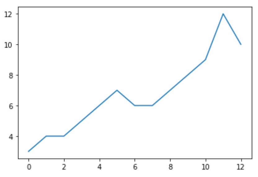 

Чтобы выполнить расширенный тест Дики-Фуллера, мы можем использовать функцию adfuller() из библиотеки statsmodels.Во-первых, нам нужно установить statsmodels:

Затем мы можем использовать следующий код для выполнения расширенного теста Дики-Фуллера:

from statsmodels. tsa.stattools import adfuller #perform augmented Dickey-Fuller test adfuller(data) (-0.9753836234744063, 0.7621363564361013, 0, 12, , 31.2466098872313) 

Вот как интерпретировать наиболее важные значения в выводе:

Поскольку p-значение не меньше 0,05, мы не можем отвергнуть нулевую гипотезу.

Это означает, что временной ряд является нестационарным. Другими словами, он имеет некоторую структуру, зависящую от времени, и не имеет постоянной дисперсии во времени.

Источник

Augmented Dickey Fuller Test (ADF Test) – Must Read Guide

Augmented Dickey Fuller test (ADF Test) is a common statistical test used to test whether a given Time series is stationary or not. It is one of the most commonly used statistical test when it comes to analyzing the stationary of a series.

1. Introduction

In ARIMA time series forecasting, the first step is to determine the number of differencing required to make the series stationary.

Since testing the stationarity of a time series is a frequently performed activity in autoregressive models, the ADF test along with KPSS test is something that you need to be fluent in when performing time series analysis.

Another point to remember is the ADF test is fundamentally a statistical significance test. That means, there is a hypothesis testing involved with a null and alternate hypothesis and as a result a test statistic is computed and p-values get reported.

It is from the test statistic and the p-value, you can make an inference as to whether a given series is stationary or not.

So, how exactly does the ADF test work? let’s see the mathematical intuition behind the test with clear examples.

2. What is a Unit Root Test?

The ADF test belongs to a category of tests called ‘Unit Root Test’, which is the proper method for testing the stationarity of a time series.

So what does a ‘Unit Root’ mean?

Unit root is a characteristic of a time series that makes it non-stationary. Technically speaking, a unit root is said to exist in a time series of the value of alpha = 1 in the below equation.

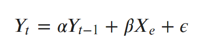
where, Yt is the value of the time series at time ‘t’ and Xe is an exogenous variable (a separate explanatory variable, which is also a time series).

What does this mean to us?

The presence of a unit root means the time series is non-stationary. Besides, the number of unit roots contained in the series corresponds to the number of differencing operations required to make the series stationary.

Alright, let’s come back to topic.

3. Dickey-Fuller Test

Before going into ADF test, let’s first understand what is the Dickey-Fuller test.

A Dickey-Fuller test is a unit root test that tests the null hypothesis that α=1 in the following model equation. alpha is the coefficient of the first lag on Y.

Null Hypothesis (H0): alpha=1

Fundamentally, it has a similar null hypothesis as the unit root test. That is, the coefficient of Y(t-1) is 1, implying the presence of a unit root. If not rejected, the series is taken to be non-stationary.

The Augmented Dickey-Fuller test evolved based on the above equation and is one of the most common form of Unit Root test.

4. How does Augmented Dickey Fuller (ADF) Test work?

As the name suggest, the ADF test is an ‘augmented’ version of the Dickey Fuller test.

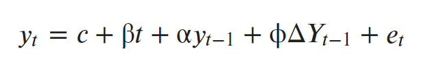
The ADF test expands the Dickey-Fuller test equation to include high order regressive process in the model.

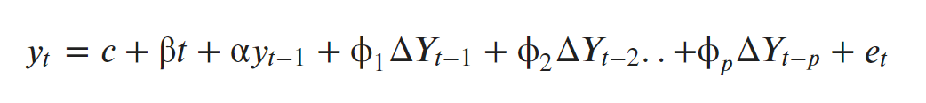
If you notice, we have only added more differencing terms, while the rest of the equation remains the same. This adds more thoroughness to the test.

The null hypothesis however is still the same as the Dickey Fuller test.

A key point to remember here is: Since the null hypothesis assumes the presence of unit root, that is α=1, the p-value obtained should be less than the significance level (say 0.05) in order to reject the null hypothesis. Thereby, inferring that the series is stationary.

However, this is a very common mistake analysts commit with this test. That is, if the p-value is less than significance level, people mistakenly take the series to be non-stationary.

5. ADF Test in Python

So, how to perform a Augmented Dickey-Fuller test in Python?

The statsmodel package provides a reliable implementation of the ADF test via the adfuller() function in statsmodels.tsa.stattools . It returns the following outputs:

1. The p-value
2. The value of the test statistic
3. Number of lags considered for the test
4. The critical value cutoffs.

When the test statistic is lower than the critical value shown, you reject the null hypothesis and infer that the time series is stationary.

Alright, let’s run the ADF test on the a10 dataset from the fpp package from R. This dataset counts the total monthly scripts for pharmaceutical products falling under ATC code A10. The original source of this dataset is the Australian Health Insurance Commission.

As see earlier, the null hypothesis of the test is the presence of unit root, that is, the series is non-stationary.

# Setup and Import data from statsmodels.tsa.stattools import adfuller import pandas as pd import numpy as np %matplotlib inline url = 'https://raw.githubusercontent.com/selva86/datasets/master/a10.csv' df = pd.read_csv(url, parse_dates=['date'], index_col='date') series = df.loc[:, 'value'].values df.plot(figsize=(14,8), legend=None, title='a10 - Drug Sales Series'); 

The packages and the data is loaded, we have everything needed to perform the test using adfuller() .

An optional argument the adfuller() accepts is the number of lags you want to consider while performing the OLS regression.

By default, this value is 12*(nobs/100)^ , where nobs is the number of observations in the series. But, optionally you can specify either the maximum number of lags with maxlags parameter or let the algorithm compute the optimal number iteratively.

This can be done by setting the autolag=’AIC’ . By doing so, the adfuller will choose a the number of lags that yields the lowest AIC. This is usually a good option to follow.

# ADF Test result = adfuller(series, autolag='AIC') print(f'ADF Statistic: ') print(f'n_lags: ') print(f'p-value: ') for key, value in result[4].items(): print('Critial Values:') print(f' , ') 

ADF Statistic: 3.1451856893067296 n_lags: 1.0 p-value: 1.0 Critial Values: 1%, -3.465620397124192 Critial Values: 5%, -2.8770397560752436 Critial Values: 10%, -2.5750324547306476 

The p-value is obtained is greater than significance level of 0.05 and the ADF statistic is higher than any of the critical values.

Clearly, there is no reason to reject the null hypothesis. So, the time series is in fact non-stationary.

6. ADF Test on stationary series

Now, let’s see another example of performing the test on a series of random numbers which is usually considered as stationary.

Let’s use np.random.randn() to generate a randomized series.

# ADF test on random numbers series = np.random.randn(100) result = adfuller(series, autolag='AIC') print(f'ADF Statistic: ') print(f'p-value: ') for key, value in result[4].items(): print('Critial Values:') print(f' , ') 

ADF Statistic: -7.4715740767231456 p-value: 5.0386184272419386e-11 Critial Values: 1%, -3.4996365338407074 Critial Values: 5%, -2.8918307730370025 Critial Values: 10%, -2.5829283377617176 

The p-value is very less than the significance level of 0.05 and hence we can reject the null hypothesis and take that the series is stationary.

Let’s visualise the series as well to confirm.

import matplotlib.pyplot as plt %matplotlib inline fig, axes = plt.subplots(figsize=(10,7)) plt.plot(series); plt.title('Random');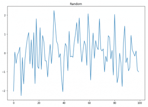 

7. Conclusion

We saw how the Augmented Dickey Fuller Test works and how to perform it using statsmodels . Now given any time series, you should be in a position to perform the ADF Test and make a fair inference on whether the series is stationary or not.

In the next one we’ll see how to perform the KPSS test.

Источник