Matplotlib: Plotting Subplots in a Loop
When carrying out exploratory data analysis (EDA), I repeatedly find myself Googling how to plot subplots in Matplotlib using a single for loop. For example, when you have a list of attributes or cross-sections of the data which you want investigate further by plotting on separate plots.
In an ideal world, you would like to be able to iterate this list of items (e.g. a list of customer IDs) and sequentially plot their values (e.g. total order value by day) on a grid of individual subplots. However, when using Matplotlib’s plotting API it is not straightforward to just create a grid of subplots and directly iterate through them in conjunction with your list of plotting attributes.
This is because, when creating the subplot grid using plt.subplots , you are returned list of lists containing the subplot objects, rather than a single list containing of subplot objects which you can iterate through in a single for loop (see below):
import matplotlib.pyplot as plt %matplotlib inline # create subplots fig, axs = plt.subplots(nrows=3, ncols=2) print(axs.shape) axs # (3, 2) # array([[, ], # [, ], # [, ]], dtype=object) 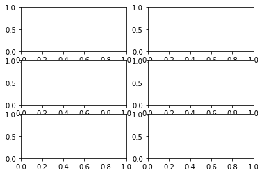
So what can we do in this situation? We have a list of items we want to plot and we have a list of lists with our subplots, is there a way to conveniently plot our data in a single for loop?
One strength, but also arguably one of Matplotlib’s biggest weaknesses, is its flexibility which allows you to accomplish the same task in many different ways. While this gives you a lot of flexibility it can be overwhelming and difficult to understand the best way to do things, particularly when starting out or learning new functionality.
In this post, I outline two different methods for plotting subplots in a single loop which I find myself using on a regular basis.
How can you loop through a subplot grid?#
Example dataset#
Before we can demonstrate the plotting methods, we need an example dataset.
For this analysis, we will use a dataset containing the daily closing stock prices of some popular tech stocks and demonstrate how to plot each time-series on a separate subplot.
Why stock prices? Because it is trendy for people to use (maybe I’ll get some good SEO?), but also using the ffn (financial functions for Python) library it is very easy to download the data for a given list of stock tickers.
The code below downloads the daily closing prices for Apple (AAPL), Microsoft (MSFT), Tesla (TSLA), Nvidia (NVDA), and Intel (INTC). Then we convert the table into long-form (one row for each datapoint) to demonstrate the plotting methods.
# library to get stock data import ffn # load daily stock prices for selected stocks from ffn tickers = ["aapl", "msft", "tsla", "nvda", "intc"] prices = ffn.get(tickers, start="2017-01-01") # convert data into a 'long' table for this plotting exercise df = prices.melt(ignore_index=False, var_name="ticker", value_name="closing_price") df.head() | ticker | closing_price | |
|---|---|---|
| Date | ||
| 2017-01-03 | aapl | 27.413372 |
| 2017-01-04 | aapl | 27.382690 |
| 2017-01-05 | aapl | 27.521944 |
| 2017-01-06 | aapl | 27.828764 |
| 2017-01-09 | aapl | 28.083660 |
Method 1: ravel() #
As the subplots are returned as a list of list, one simple method is to ‘flatten’ the nested list into a single list using NumPy’s ravel() (or flatten()) method.
Here we iterate the tickers list and the axes lists at the same time using Python’s zip function and using ax.ravel() to flatten the original list of lists. This allows us to iterate the axes as if they are a simple list.
# define subplot grid fig, axs = plt.subplots(nrows=3, ncols=2, figsize=(15, 12)) plt.subplots_adjust(hspace=0.5) fig.suptitle("Daily closing prices", fontsize=18, y=0.95) # loop through tickers and axes for ticker, ax in zip(tickers, axs.ravel()): # filter df for ticker and plot on specified axes df[df["ticker"] == ticker].plot(ax=ax) # chart formatting ax.set_title(ticker.upper()) ax.get_legend().remove() ax.set_xlabel("") plt.show() 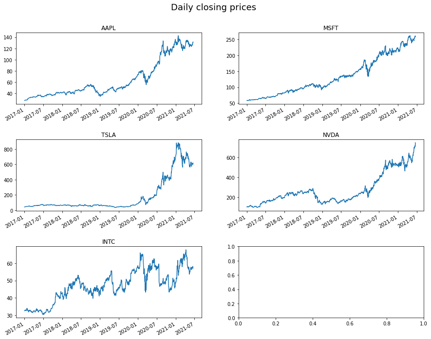
Great! So we can now plot each time-series on independent subplots.
However, you will notice a slight issue — there is an annoying empty plot at the end. This is because we have five tickers but we specified a 3×2 subplot grid (6 in total) so there is an unnecessary plot left over.
A downside of the ravel() approach is that we specify and create the entire subplot grid first, and then add the plotting data to each plot in turn. Once we have run out of things to plot, we stop adding data to the subplots regardless of whether all the subplots have been used. This means if you have an odd number of inputs (as we have in our case), then you will have empty plots left over. Luckily, there is another approach…
Note
You could remove this empty plot after the fact by deleting it – for example using fig.delaxes(axes[2][1]) . However, I find this a less satisfactory solution which could get complicated quickly. For example, if there are multiple empty plots that you don’t know ahead of time.
Method 2: plt.subplot #
An alternative approach is to create an axis object on the fly inside the loop, although you still need to specify the grid size (rows x cols) ahead of time.
This means that you only create an axis if there is data to fill it and you do not get unnecessary empty plots.
plt.figure(figsize=(15, 12)) plt.subplots_adjust(hspace=0.5) plt.suptitle("Daily closing prices", fontsize=18, y=0.95) # loop through the length of tickers and keep track of index for n, ticker in enumerate(tickers): # add a new subplot iteratively ax = plt.subplot(3, 2, n + 1) # filter df and plot ticker on the new subplot axis df[df["ticker"] == ticker].plot(ax=ax) # chart formatting ax.set_title(ticker.upper()) ax.get_legend().remove() ax.set_xlabel("") 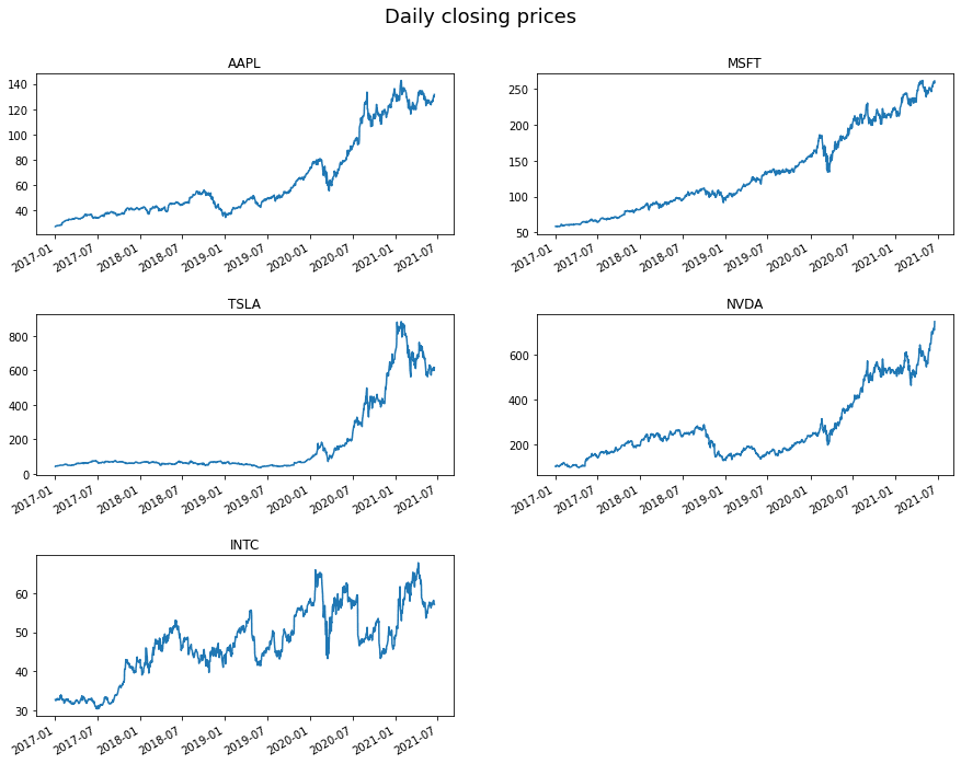
Here we used the plt.subplot syntax inside the loop and specified which subplot index we should plot the data. We used Python’s enumerate function so we could record the index position (n) of the list as we iterate it. We need to add 1 to this number as enumerate starts counting from zero, but plt.subplot starts counting at 1.
So which method should you use?#
Method 2 is probably the most generally applicable as it does not rely on an even number of inputs.
I still tend to use both as I find method 1 syntax easier to remember — maybe it is something confusing about the plt.subplots vs plt.subplot notation in method 2 — but use method 2 if there is an odd number of inputs.
A downside to both methods is that you need to specify the grid size ahead of time. This means you need to know the length of the input list of (in our case) tickers, which might not always be possible (e.g. if using generators instead of lists). However, in most cases this is not a problem.
Improvements: Dynamic Grid Sizing#
In the examples above, we have hard-coded the number of rows and columns for the subplot grid. Wouldn’t it be better if we could generate this information dynamically? For example, if the length of the inputs became longer in the future.
If we calculate the length of the list we are iterating through, we can find the required grid dimensions using the snippet below to dynamically calculate the minimum number of rows in a grid.
# find minimium required rows given we want 2 columns ncols = 2 nrows = len(tickers) // ncols + (len(tickers) % ncols > 0) ## nrows ## 3 Here we specify the number of columns we want and the code will evaluate the minimum number of rows required. This functionality is useful if you want to change the number of columns for your plots at a later date or if you want to allow for a more generalised approach.
The code below demonstrates how easy it is to change the grid layout to three columns instead of two, by changing the ncols variable value.
plt.figure(figsize=(15, 12)) plt.subplots_adjust(hspace=0.2) plt.suptitle("Daily closing prices", fontsize=18, y=0.95) # set number of columns (use 3 to demonstrate the change) ncols = 3 # calculate number of rows nrows = len(tickers) // ncols + (len(tickers) % ncols > 0) # loop through the length of tickers and keep track of index for n, ticker in enumerate(tickers): # add a new subplot iteratively using nrows and cols ax = plt.subplot(nrows, ncols, n + 1) # filter df and plot ticker on the new subplot axis df[df["ticker"] == ticker].plot(ax=ax) # chart formatting ax.set_title(ticker.upper()) ax.get_legend().remove() ax.set_xlabel("") 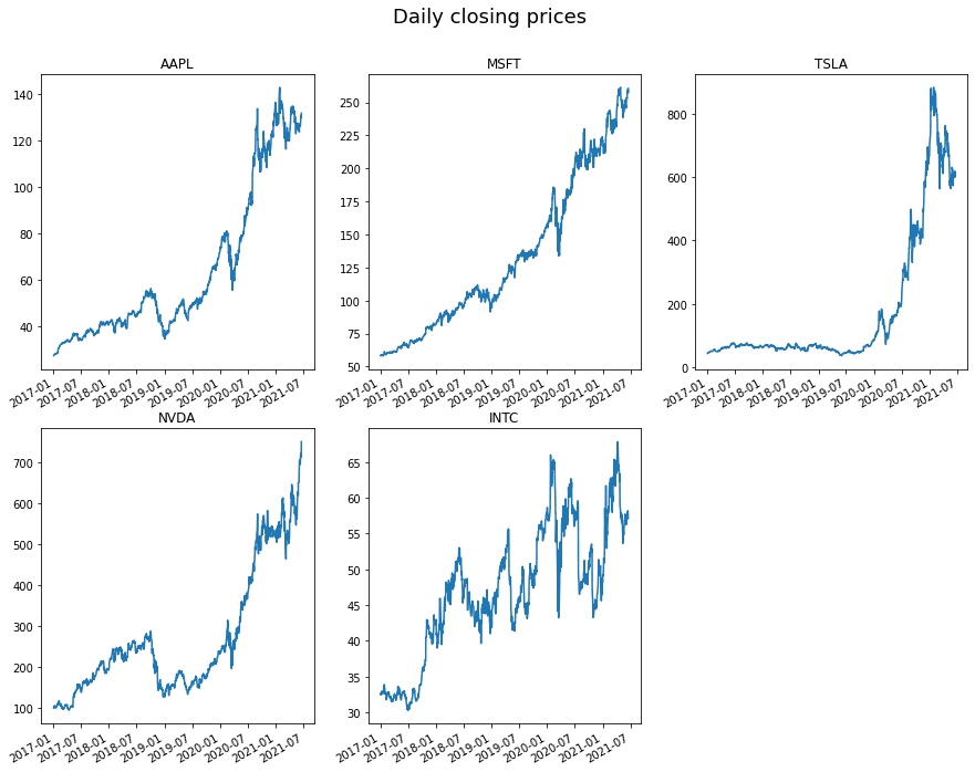
Other Methods#
This example is slightly contrived because there are inbuilt methods in Pandas that will do this for you. E.g. using df.groupby(‘ticker’).plot() , however, you may not have as much easy control over chart formatting.
Equally you could also use Seaborn, however, the API for subplots (Facet grids ) can be just as cumbersome.
Conclusion#
In this post, we have demonstrated two different methods for plotting subplot grids using a for loop. Like many things in programming, the best solution will depend on your specific use case, but this post has described a number of options.
Normally it is best to use Pandas inbuilt plotting functions where possible, however, if you need something a little more custom, methods 1 and 2 described here could help.
⭐Top tip
Save little snippets like this in a central repository you can access for future projects – it will save a bunch of time
Resources and References#
- Engineering for Data Science Github
- Accompanying Notebook
- Matplotlib documentation
- Tensorflow image classification tutorials – you can see some good examples of how to plot images in a grid!
Further Reading#
Find value in this article? Please help this blog by sharing using the icons below — 🍻 cheers!