Построение линии тренда python

Python – How to Add Trend Line to Line Chart / Graph

In this plot, you will learn about how to add trend line to the line chart / line graph using Python Matplotlib.As a data scientist, it proves to be helpful to learn the concepts and related Python code which can be used to draw or add the trend line to the line charts as it helps understand the trend and make decisions.

In this post, we will consider an example of IPL average batting scores of Virat Kohli, Chris Gayle, MS Dhoni and Rohit Sharma of last 10 years, and, assess the trend related to their overall performance using trend lines. Let’s say that main reason why we want to understand the trend line? The primary goal is to assess on whom could the larger money be put in order to acquire him for the team? The batsman who has the largest upward trend line with highest slope is the one I would like to put my money on. Having said that, the batting scores mean and variance / standard deviation also comes into picture in taking the final decision on who to put larger money on.

Here is their batting average scores in IPL seasons in last 10 years from 2010 – 2019

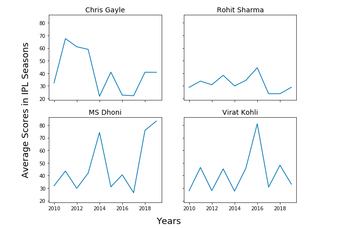
You may note that it becomes difficult to find out about the performance of batsman across different seasons. Thus, if one would like to make a decision on who to put larger money on to acquire for the next season, IPL 2020 (currently going on), it would just get difficult.

This is where adding trend line to all of the line charts will make difference.

How to draw trend line for line chart / graph using Python?

First and foremost, lets represent the IPL batting average scores data across different seasons from 2010-2019 shown in table 1 in form of numpy array.

import numpy as np # # Chris Gayle # chris_gayle = np.array([32.44, 67.55, 61.08, 59.00, 21.77, 40.91, 22.70, 22.22, 40.88, 40.83]) # # Rohit Sharma # rohit_sharma = np.array([28.85, 33.81, 30.92, 38.42, 30.00, 34.42, 44.45, 23.78, 23.83, 28.92]) # # MS Dhoni # ms_dhoni = np.array([31.88, 43.55, 29.83, 41.90, 74.20, 31.00, 40.57, 26.36, 75.83, 83.20]) # # Virat Kohli # virat_kohli = np.array([27.90, 46.41, 28.00, 45.28, 27.61, 45.90, 81.08, 30.80, 48.18, 33.14])

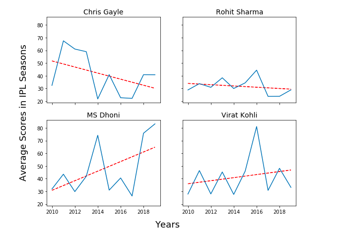
Here is the Python code which is used to draw the trend lines for line charts / line graphs in order to assess the overall performance of these batsman in last 10 years in terms of increasing or decreasing scoring trends.

import matplotlib.pyplot as plt import numpy as np # # Number of years represented as Numpy Array # X = np.array([2010, 2011, 2012, 2013, 2014, 2015, 2016, 2017, 2018, 2019]) fig, ax = plt.subplots(2, 2, figsize=(9, 7), sharex=True, sharey=True) # # Chris Gayle # z = np.polyfit(X, chris_gayle, 1) p = np.poly1d(z) ax[1, 0].plot(X,p(X),"r--") ax[1, 0].plot(X, chris_gayle) ax[1, 0].set_title('Chris Gayle', fontsize=14) # # Rohit Sharma # z = np.polyfit(X, rohit_sharma, 1) p = np.poly1d(z) ax[0, 0].plot(X,p(X),"r--") ax[0, 0].plot(X, rohit_sharma ) ax[0, 0].set_title('Rohit Sharma', fontsize=14) # # MS Dhoni # z = np.polyfit(X, ms_dhoni, 1) p = np.poly1d(z) ax[1, 1].plot(X,p(X),"r--") ax[1, 1].plot(X, ms_dhoni) ax[1, 1].set_title('MS Dhoni', fontsize=14) # # Virat Kohli # z = np.polyfit(X, virat_kohli, 1) p = np.poly1d(z) ax[0, 1].plot(X,p(X),"r--") ax[0, 1].plot(X, virat_kohli) ax[0, 1].set_title('Virat Kohli', fontsize=14) # # Draw the plot # fig.text(0.5, 0.04, 'Years', ha='center', fontsize=18) fig.text(0.04, 0.5, 'Average Scores in IPL Seasons', va='center', rotation='vertical', fontsize=18)

Here is how the trend line plot would look like for all the players listed in this post.

The Python code which does the magic of drawing / adding the trend line to the line chart / line graph is the following. Pay attention to some of the following in the code given below:

• Two plots have been created – One is Line chart / line plot / line graph, and, other is trend line.
• Plotting code which represents line chart is ax[0, 1].plot(X, virat_kohli)
• Plotting code which represents trend line is the following. Numpy ployfit method is used to fit the trend line which then returns the coefficients.

z = np.polyfit(X, virat_kohli, 1) // Polynomial fit p = np.poly1d(z) ax[0, 1].plot(X,p(X),"r--")

Here is the full Python code for adding trend line to the line chart.

virat_kohli = np.array([27.90, 46.41, 28.00, 45.28, 27.61, 45.90, 81.08, 30.80, 48.18, 33.14]) z = np.polyfit(X, virat_kohli, 1) // Polynomial fit p = np.poly1d(z) ax[0, 1].plot(X,p(X),"r--") ax[0, 1].plot(X, virat_kohli) ax[0, 1].set_title('Virat Kohli', fontsize=14)

Line Chart & Trend line Analysis

Given the trend line in figure 2, it can be concluded that MS Dhoni batting averages have been increasing as it has upward trend line. That said, Virat Kohli batting average also has upward trend line but the slope is lesser than that of MS Dhoni. Thus, if it comes to take decision on who to put larger money on, I would bet my money on MS Dhoni.

Conclusions

Here is the summary of what you learned about adding trend line to line graph or line chart using Python:

• Matplotlib can be used to draw line chart and trend line
• Matplotlib plot function is used to draw the line chart and trend line
• Numpy ployfit method is used to fit the polynomial which returns coefficients which are later used to draw the trend line.

Ajitesh Kumar

I have been recently working in the area of Data analytics including Data Science and Machine Learning / Deep Learning. I am also passionate about different technologies including programming languages such as Java/JEE, Javascript, Python, R, Julia, etc, and technologies such as Blockchain, mobile computing, cloud-native technologies, application security, cloud computing platforms, big data, etc. For latest updates and blogs, follow us on Twitter. I would love to connect with you on Linkedin. Check out my latest book titled as First Principles Thinking: Building winning products using first principles thinking

Источник

Как добавить линию тренда в Matplotlib (с примером)

Вы можете использовать следующий базовый синтаксис, чтобы добавить линию тренда на график в Matplotlib:

#create scatterplot plt.scatter (x, y) #calculate equation for trendline z = np.polyfit (x, y, 1) p = np.poly1d (z) #add trendline to plot plt.plot (x, p(x)) 

В следующих примерах показано, как использовать этот синтаксис на практике.

Пример 1: создание линейной линии тренда в Matplotlib

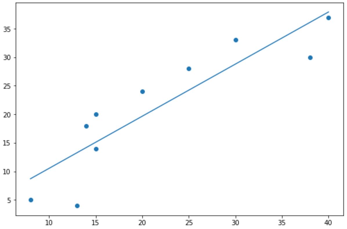
В следующем коде показано, как создать базовую линию тренда для диаграммы рассеяния в Matplotlib:

import numpy as np import matplotlib.pyplot as plt #define data x = np.array([8, 13, 14, 15, 15, 20, 25, 30, 38, 40]) y = np.array([5, 4, 18, 14, 20, 24, 28, 33, 30, 37]) #create scatterplot plt.scatter (x, y) #calculate equation for trendline z = np.polyfit (x, y, 1 ) p = np.poly1d (z) #add trendline to plot plt.plot (x, p(x)) 

Синие точки представляют точки данных, а прямая синяя линия представляет собой линейную линию тренда.

Обратите внимание, что вы также можете использовать аргументы color , linewidth и linestyle для изменения внешнего вида линии тренда:

#add custom trendline to plot plt.plot (x, p(x), color=" purple", linewidth= 3 , linestyle=" -- ")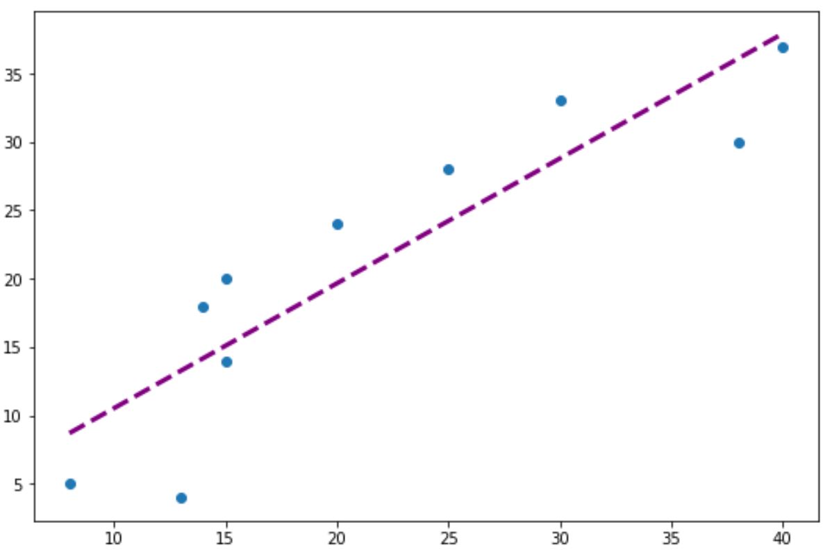 

Пример 2: создание полиномиальной линии тренда в Matplotlib

Чтобы создать полиномиальную линию тренда, просто измените значение в функции np.polyfit() .

Например, мы могли бы использовать значение 2 для создания квадратичной линии тренда:

import numpy as np import matplotlib.pyplot as plt #define data x = np.array([8, 13, 14, 15, 15, 20, 25, 30, 38, 40]) y = np.array([5, 4, 18, 14, 20, 24, 28, 33, 30, 37]) #create scatterplot plt.scatter (x, y) #calculate equation for quadratic trendline z = np.polyfit (x, y, 2 ) p = np.poly1d (z) #add trendline to plot plt.plot (x, p(x))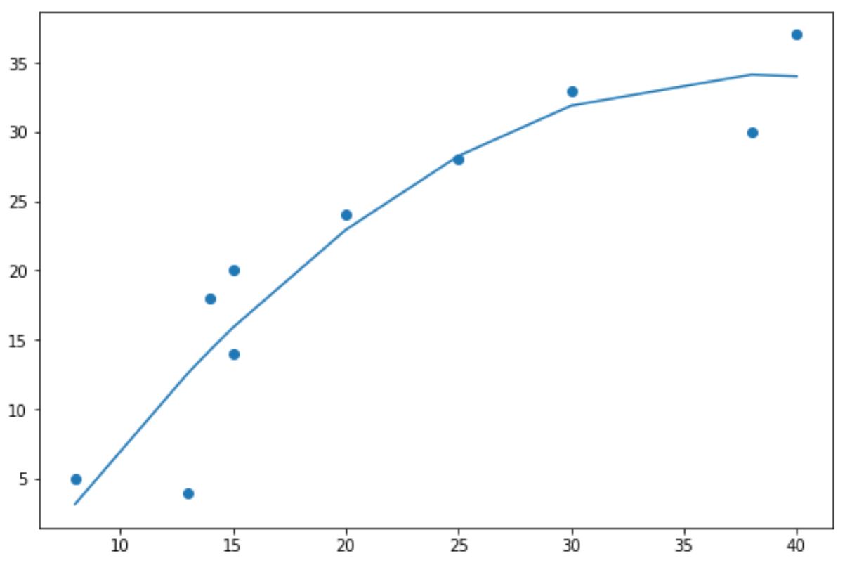 

Обратите внимание, что линия тренда теперь изогнута, а не прямая.

Эта полиномиальная линия тренда особенно полезна, когда ваши данные демонстрируют нелинейный шаблон, а прямая линия плохо отражает тренд в данных.

Дополнительные ресурсы

В следующих руководствах объясняется, как выполнять другие распространенные функции в Matplotlib:

Источник

techflare

tech trends and hands-on, flaring enthusiasm for building blocks

How to draw a trend line with DataFrame in Python

DataScience

Python

A trendline is a line drawn over pivot highs or under pivot lows to show the prevailing direction of price.

A trend line is one of important tools for technical traders. Trandline’s vidualization is recognizable for traders to know a direction of trend and patterns of price bounces. During the analyzed timeframe, analysts take at least 2 points in a chart to connect those points to draw a straight line.

When you take lower points in a trend, a trend like acts like a support line while taken higher points can act like a resistence line in a trend. So it can be employed to know these 2 points in a chart.

Let’s assume we have 2 lower price points in a chart and draw a trend line. When the current price hits this uptrend line, the price curve might be rebounced within the trend. Or if the price breaks under the uptrend line drawn with the lower points, it can be thought of as a price pivot to bearlish.

Now if we have 2 higher price points in a chart and we draw a trend line by connecting 2 points. When the current price hits the downtrend line, the price curve might be rebounced within the trend. Or if the breaks above the downtrend line drawn with the higher points, it can be thought of as a price pivot to bullish.

To compute technical indicators in Python, we have Ta-lib and pyti libraries but a trend line and support/resistence lines are not included to calculate in those libraries. In this article, I’d like to show how to write trend lines from DataFrame object in matplotlib, Python.

To obtain return data of your portfolio or securities please refer to the previous writing. In this blog it’s explained to retrieve stock data in Pandas Datareader (All codes are there) and how to compute daily returns and cumulative returns over a certain period of time such as daily, weekly, monthly and yearly.

Simple linear regression

As mentioned, the basic drawing of trendlines is to connect at least 2 points in a chart. Let’s deem this problem as a simple linear regression, then we can use scipy.stats.linregress method that calculates a linear least-squares regression for two sets of measurements. Let’s take a look at the sample.

We have 2 blue points (2, 5) and (7, 15) in this euclidean plane. scipy.stats.linregress can fit a straight line computed from these points (the red line in this graph). The method returns a slope, interception, p&r values also standard errors.

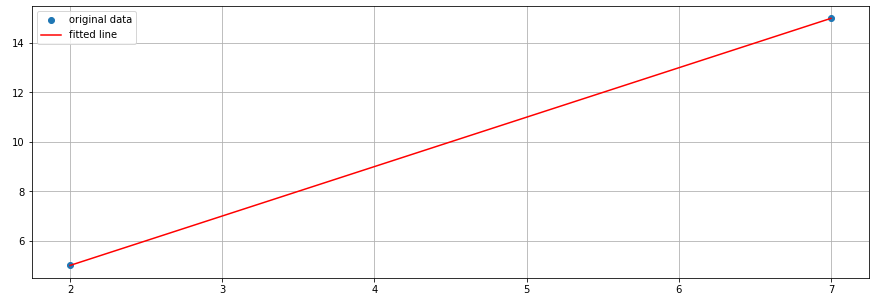
Here’s the code how to draw this graph and the regression line. Let’s use a similar code for drawing trend lines in the following section.

Here are the code snippet how to pick up 2 higher and lower data points from DataFrame. The computation returned only 2 sets of DataFrame rows where the data points broke above or below the calculated linear regression line in either case.

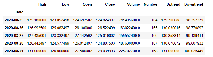
At last, we can use line plot of matplotlib with the 3 columns. 1 is the Close data to draw the closing price in green. The rest 2 of 3 are Uptrend and Downtrend that were calculated from scipy.stats.linregress to fit a straight line between 2 higher points or 2 lower points.

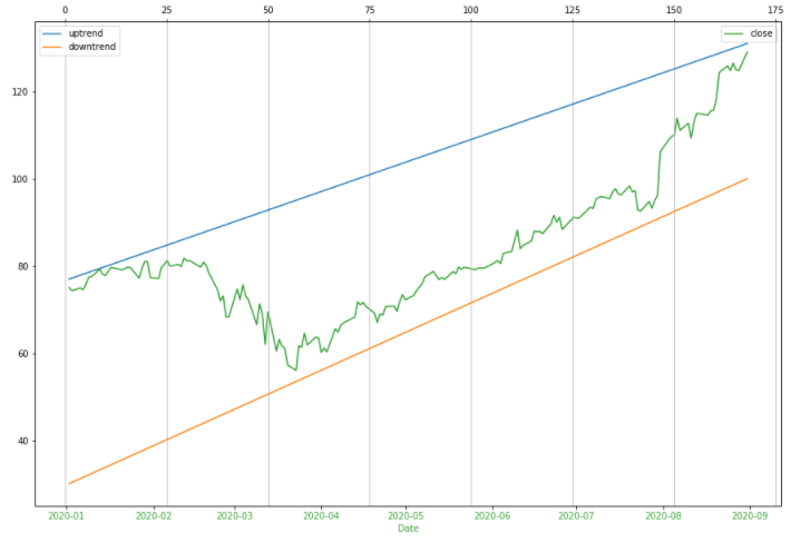
Actually this example doesn’t so look good so you can apply the same method for other assets or different time scales and timeframes.

Here’s the Jupyter notebook of all samples in github for your reference.

Источник