Построение фазовых портретов python

Phase Portraits¶

In this notebook we’ll look at how to generate phase portraits. A phase diagram shows the trajectories that a dynamical system can take through its phase space. For any system that obeys the markov property we can construct such a diagram, with one dimension for each of the system’s stocks.

Ingredients¶

Libraries¶

In this analysis we’ll use:

• numpy to create the grid of points that we’ll sample over
• matplotlib via ipython’s pylab magic to construct the quiver plot

%pylab inline import pysd import numpy as np 

Populating the interactive namespace from numpy and matplotlib 

Example Model¶

A single pendulum makes for a great example of oscillatory behavior. The following model constructs equations of motion for the pendulum in radial coordinates, simplifying the model from one constructed in cartesian coordinates. In this model, the two state elements are the angle of the pendulum and the derivative of that angle, its angular velocity.

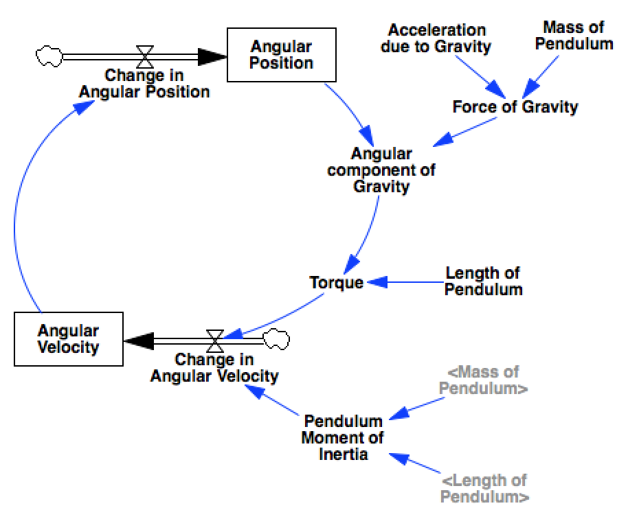
model = pysd.read_vensim('../../models/Pendulum/Single_Pendulum.mdl') 

Recipe¶

Step 1: Define the range over which to plot¶

We’ve defined the angle \(0\) to imply that the pendulum is hanging straight down. To show the full range of motion, we’ll show the angles ragning from \(-1.5\pi\) to \(+1.5\pi\) , which will allow us to see the the points of stable and unstable equilibrium.

We also want to sample over a range of angular velocities that are reasonable for our system, for the given values of length and weight.

angular_position = np.linspace(-1.5*np.pi, 1.5*np.pi, 60) angular_velocity = np.linspace(-2, 2, 20) 

Numpy’s meshgrid lets us construct a 2d sample space based upon our arrays

apv, avv = np.meshgrid(angular_position, angular_velocity) 

Step 2: Calculate the state space derivatives at a point¶

We’ll define a helper function, which given a point in the state space, will tell us what the derivatives of the state elements will be. One way to do this is to run the model over a single timestep, and extract the derivative information. In this case, the model’s stocks have only one inflow/outflow, so this is the derivative value.

As the derivative of the angular position is just the angular velocity, whatever we pass in for the av parameter should be returned to us as the derivative of ap .

def derivatives(ap, av): ret = model.run(params='angular_position':ap, 'angular_velocity':av>, return_timestamps=[0,1], return_columns=['change_in_angular_position', 'change_in_angular_velocity']) return tuple(ret.loc[0].values) derivatives(0,1) 

Step 3: Calculate the state space derivatives across our sample space¶

We can use numpy’s vectorize to make the function accept the 2d sample space we have just created. Now we can generate the derivative of angular position vector dapv and that of the angular velocity vector davv . As before, the derivative of the angular posiiton should be equal to the angular velocity. We check that the vectors are equal.

vderivatives = np.vectorize(derivatives) dapv, davv = vderivatives(apv, avv) (dapv == avv).all() 

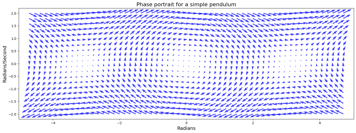
Step 4: Plot the phase portrait¶

Now we have everything we need to draw the phase portrait. We’ll use matplotlib’s quiver function, which wants as arguments the grid of x and y coordinates, and the derivatives of these coordinates.

In the plot we see the locations of stable and unstable equilibria, and can eyeball the trajectories that the system will take through the state space by following the arrows.

plt.figure(figsize=(18,6)) plt.quiver(apv, avv, dapv, davv, color='b', alpha=.75) plt.box('off') plt.xlim(-1.6*np.pi, 1.6*np.pi) plt.xlabel('Radians', fontsize=14) plt.ylabel('Radians/Second', fontsize=14) plt.title('Phase portrait for a simple pendulum', fontsize=16); 

© Copyright 2015, James Houghton. Revision 23c6f9a3 .

Versions latest Downloads pdf htmlzip epub On Read the Docs Project Home Builds Free document hosting provided by Read the Docs.

Источник

Installation

Phaseportrait releases are available as wheel packages for macOS, Windows and Linux on PyPI. Install it using pip:

$ pip install phaseportrait 

Installing from source:

Open a terminal on desired route and type the following:

$ git clone https://github.com/phaseportrait/phaseportrait 

Manual installation

Visit phase-portrait webpage on GitHub. Click on green button saying Code, and download it in zip format. Save and unzip on desired directory.

What’s this?

The idea behind this project was to create a simple way to make phase portraits in 2D and 3D in Python, as we couldn’t find something similar on the internet, so we got down to work. (Update: found jmoy/plotdf, offers similar 2D phase plots but it is very limited).

Eventually, we did some work on bifurcations, 1D maps and chaos in 3D trayectories.

This idea came while taking a course in non linear dynamics and chaos, during the 3rd year of physics degree, brought by our desire of visualizing things and programming.

We want to state that we are self-taught into making this kind of stuff, and we’ve tried to make things as professionally as possible, any comments about improving our work are welcome!

Authors

Contributing

This proyect is open-source, everyone can download, use and contribute. To do that, several options are offered:

• Fork the project, add a new feature / improve the existing ones and pull a request via GitHub.
• Contact us on our emails:
  • vhloras@gmail.com
  • unaileria@gmail.com

  Источник

  Digiratory

  Лаборатория автоматизации и цифровой обработки сигналов

  

  Построение фазовых портретов на языке Python

  Фазовая траектория — след от движения изображающей точки. Фазовый портрет — это полная совокупность различных фазовых траекторий. Он хорошо иллюстрирует поведение системы и основные ее свойства, такие как точки равновесия.

  С помощью фазовых портретов можно синтезировать регуляторы (Метод фазовой плоскости) или проводить анализ положений устойчивости и характера движений системы.

  Рассмотрим построение фазовых портретов нелинейных динамических систем, представленных в форме обыкновенных дифференциальных уравнений

  В качестве примера воспользуемся моделью маятника с вязким трением:

  Где \(\omega \) — скорость, \(\theta \) — угол отклонения, \(b \) — коэффициент вязкого трения, \(с \) — коэффициент, учитывающий массу, длину и силу тяжести.

  Для работы будем использовать библиотеки numpy, scipy и matplotlib для языка Python.

  Блок импорта выглядит следующим образом:

  import numpy as np from scipy.integrate import odeint import matplotlib.pyplot as plt

  Шаг 1. Реализация ОДУ в Python

  Определим функцию, отвечающую за расчет ОДУ. Например, следующего вида:

  def ode(y, t, b, c): theta, omega = y dydt = [omega, -b*omega - c*np.sin(theta)] return dydt

  Аргументами функции являются:

  • y — вектор переменных состояния
  • t — время
  • b, c — параметры ДУ (может быть любое количество)

  Функция возвращает вектор производных.

  Шаг 2. Численное решение ОДУ

  Далее необходимо реализовать функцию для получения решения ОДУ с заданными начальными условиями:

  def calcODE(args, y0, dy0, ts = 10, nt = 101): y0 = [y0, dy0] t = np.linspace(0, ts, nt) sol = odeint(ode, y0, t, args) return sol

  Аргументами функции являются:

  • args — Параметры ОДУ (см. шаг 1)
  • y0— Начальные условия для первой переменной состояния
  • dy0 — Начальные условия для второй переменной состояния (или в нашем случае ее производной)
  • ts — длительность решения
  • nt — Количество шагов в решении (= время интегрирования * шаг времени)

  В 3-й строке формируется вектор временных отсчетов. В 4-й строке вызывается функция решения ОДУ.

  Шаг 3. Генерация и вывод фазового портрета

  Для построения фазового портрета необходимо произвести решения ОДУ с различными начальными условиями (вокруг интересующей точки). Для реализации также напишем функцию.

  def drawPhasePortrait(args, deltaX = 1, deltaDX = 1, startX = 0, stopX = 5, startDX = 0, stopDX = 5, ts = 10, nt = 101): for y0 in range(startX, stopX, deltaX): for dy0 in range(startDX, stopDX, deltaDX): sol = calcODE(args, y0, dy0, ts, nt) plt.plot(sol[:, 1], sol[:, 0], 'b') plt.xlabel('x') plt.ylabel('dx/dt') plt.grid() plt.show()

  Аргументами функции являются:

  • args — Параметры ОДУ (см. шаг 1)
  • deltaX — Шаг начальных условий по горизонтальной оси (переменной состояния)
  • deltaDX — Шаг начальных условий по вертикальной оси (производной переменной состояния)
  • startX — Начальное значение интервала начальных условий
  • stopX — Конечное значение интервала начальных условий
  • startDX — Начальное значение интервала начальных условий
  • stopDX — Конечное значение интервала начальных условий
  • ts — длительность решения
  • nt — Количество шагов в решении (= время интегрирования * шаг времени)

  Во вложенных циклах (строки 3-4) происходит перебор начальных условий дифференциального уравнения. В теле этих циклов (строки 5-6) происходит вызов функции решения ОДУ с заданными НУ и вывод фазовая траектории полученного решения.

  Далее производятся нехитрые действия:

  • Строка 7 — задается название оси X
  • Строка 9 — задается название оси Y
  • Строка 10 — выводится сетка на графике
  • Строка 11 — вывод графика (рендер)

  Шаг 4. Запуск построения

  Запустить построение можно следующим образом:

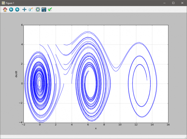
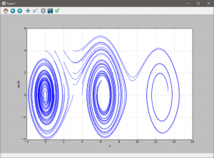
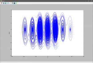
  b = 0.25 c = 5.0 args=(b, c) drawPhasePortrait(args) drawPhasePortrait(args, 1, 1, -10, 10, -5, 5, ts = 30, nt = 301)

  Строка 1-2 — задание значений параметрам ОДУ

  Строка 3 — формирование вектора параметров

  Строка 4 — вызов функции генерации фазового портрета с параметрами «по умолчанию»

  Строка 5 — вызов функции генерации фазового портрета с настроенными параметрами

  Итог

  При запуске программы получаем следующий результат:

  

  

  Полный текст программы под лицензией MIT (Использование при условии ссылки на источник):

  # -*- coding: utf-8 -*- """ This function create a phase portrait of ode Created on Mon Jan 23 18:51:01 2017 Copyright 2017 Sinitsa AM site: digiratory.ru Permission is hereby granted, free of charge, to any person obtaining a copy of this software and associated documentation files (the "Software"), to deal in the Software without restriction, including without limitation the rights to use, copy, modify, merge, publish, distribute, sublicense, and/or sell copies of the Software, and to permit persons to whom the Software is furnished to do so, subject to the following conditions: The above copyright notice and this permission notice shall be included in all copies or substantial portions of the Software. THE SOFTWARE IS PROVIDED "AS IS", WITHOUT WARRANTY OF ANY KIND, EXPRESS OR IMPLIED, INCLUDING BUT NOT LIMITED TO THE WARRANTIES OF MERCHANTABILITY, FITNESS FOR A PARTICULAR PURPOSE AND NONINFRINGEMENT. IN NO EVENT SHALL THE AUTHORS OR COPYRIGHT HOLDERS BE LIABLE FOR ANY CLAIM, DAMAGES OR OTHER LIABILITY, WHETHER IN AN ACTION OF CONTRACT, TORT OR OTHERWISE, ARISING FROM, OUT OF OR IN CONNECTION WITH THE SOFTWARE OR THE USE OR OTHER DEALINGS IN THE SOFTWARE. @author: Sinitsa AM digiratory.ru """ import numpy as np from scipy.integrate import odeint import matplotlib.pyplot as plt ''' In this function you should implement your ode for example: d*theta/dt = omega d*omega/dt = -b*omega - c*np.sin(theta) @args: y - state variable t - time b, c - args of ode ''' def ode(y, t, b, c): theta, omega = y dydt = [omega, -b*omega - c*np.sin(theta)] return dydt ''' Calculate ode @args: args - arguments of ODE y0 - The initial state of y yd0 - The initial state of derivative y ts - the duration of the simulation nt - Number steps if simulation (=ts*deltat) ''' def calcODE(args, y0, dy0, ts = 10, nt = 101): y0 = [y0, dy0] t = np.linspace(0, ts, nt) sol = odeint(ode, y0, t, args) return sol ''' Drawing Phase portrait of ODE in function ode() @args: args - arguments of ODE deltaX - step x deltaDX - step derivative x startX - start value of x stopX - stop value of x startDX - start value of derivative x stopDX - stop value of derivative x ts - the duration of the simulation nt - Number steps if simulation (=ts*deltat) ''' def drawPhasePortrait(args, deltaX = 1, deltaDX = 1, startX = 0, stopX = 5, startDX = 0, stopDX = 5, ts = 10, nt = 101): for y0 in range(startX, stopX, deltaX): for dy0 in range(startDX, stopDX, deltaDX): sol = calcODE(args, y0, dy0, ts, nt) plt.plot(sol[:, 0], sol[:, 1], 'b') plt.xlabel('x') plt.ylabel('dx/dt') plt.grid() plt.show() b = 0.25 c = 5.0 args=(b, c) drawPhasePortrait(args) drawPhasePortrait(args, 1, 1, -10, 10, -5, 5, ts = 30, nt = 301)

  Синица А.М.: Построение фазовых портретов на языке Python [Электронный ресурс] // Digiratory. 2017 г. URL: https://digiratory.ru/?p=435 (дата обращения: ДД.ММ.ГГГГ).

  Построение фазовых портретов на языке Python : 2 комментария

  Источник