Plt plot python прозрачность

Specifying colors#

Matplotlib recognizes the following formats to specify a color.

RGB or RGBA (red, green, blue, alpha) tuple of float values in a closed interval [0, 1].

Case-insensitive hex RGB or RGBA string.

Case-insensitive RGB or RGBA string equivalent hex shorthand of duplicated characters.

String representation of float value in closed interval [0, 1] for grayscale values.

Single character shorthand notation for some basic colors.

The colors green, cyan, magenta, and yellow do not coincide with X11/CSS4 colors. Their particular shades were chosen for better visibility of colored lines against typical backgrounds.

• ‘b’ as blue
• ‘g’ as green
• ‘r’ as red
• ‘c’ as cyan
• ‘m’ as magenta
• ‘y’ as yellow
• ‘k’ as black
• ‘w’ as white

Case-insensitive X11/CSS4 color name with no spaces.

Case-insensitive color name from xkcd color survey with ‘xkcd:’ prefix.

Case-insensitive Tableau Colors from ‘T10’ categorical palette.

This is the default color cycle.

• ‘tab:blue’
• ‘tab:orange’
• ‘tab:green’
• ‘tab:red’
• ‘tab:purple’
• ‘tab:brown’
• ‘tab:pink’
• ‘tab:gray’
• ‘tab:olive’
• ‘tab:cyan’

«CN» color spec where ‘C’ precedes a number acting as an index into the default property cycle.

Matplotlib indexes color at draw time and defaults to black if cycle does not include color.

rcParams[«axes.prop_cycle»] (default: cycler(‘color’, [‘#1f77b4’, ‘#ff7f0e’, ‘#2ca02c’, ‘#d62728’, ‘#9467bd’, ‘#8c564b’, ‘#e377c2’, ‘#7f7f7f’, ‘#bcbd22’, ‘#17becf’]) )

«Red», «Green», and «Blue» are the intensities of those colors. In combination, they represent the colorspace.

Transparency#

The alpha value of a color specifies its transparency, where 0 is fully transparent and 1 is fully opaque. When a color is semi-transparent, the background color will show through.

The alpha value determines the resulting color by blending the foreground color with the background color according to the formula

The following plot illustrates the effect of transparency.

import matplotlib.pyplot as plt from matplotlib.patches import Rectangle import numpy as np fig, ax = plt.subplots(figsize=(6.5, 1.65), layout='constrained') ax.add_patch(Rectangle((-0.2, -0.35), 11.2, 0.7, color='C1', alpha=0.8)) for i, alpha in enumerate(np.linspace(0, 1, 11)): ax.add_patch(Rectangle((i, 0.05), 0.8, 0.6, alpha=alpha, zorder=0)) ax.text(i+0.4, 0.85, f"alpha:.1f>", ha='center') ax.add_patch(Rectangle((i, -0.05), 0.8, -0.6, alpha=alpha, zorder=2)) ax.set_xlim(-0.2, 13) ax.set_ylim(-1, 1) ax.set_title('alpha values') ax.text(11.3, 0.6, 'zorder=1', va='center', color='C0') ax.text(11.3, 0, 'zorder=2\nalpha=0.8', va='center', color='C1') ax.text(11.3, -0.6, 'zorder=3', va='center', color='C0') ax.axis('off') 

The orange rectangle is semi-transparent with alpha = 0.8. The top row of blue squares is drawn below and the bottom row of blue squares is drawn on top of the orange rectangle.

See also Zorder Demo to learn more on the drawing order.

«CN» color selection#

Matplotlib converts «CN» colors to RGBA when drawing Artists. The Styling with cycler section contains additional information about controlling colors and style properties.

import numpy as np import matplotlib.pyplot as plt import matplotlib as mpl th = np.linspace(0, 2*np.pi, 128) def demo(sty): mpl.style.use(sty) fig, ax = plt.subplots(figsize=(3, 3)) ax.set_title('style: '.format(sty), color='C0') ax.plot(th, np.cos(th), 'C1', label='C1') ax.plot(th, np.sin(th), 'C2', label='C2') ax.legend() demo('default') demo('seaborn-v0_8') 

• 
• 

The first color ‘C0’ is the title. Each plot uses the second and third colors of each style’s rcParams[«axes.prop_cycle»] (default: cycler(‘color’, [‘#1f77b4’, ‘#ff7f0e’, ‘#2ca02c’, ‘#d62728’, ‘#9467bd’, ‘#8c564b’, ‘#e377c2’, ‘#7f7f7f’, ‘#bcbd22’, ‘#17becf’]) ). They are ‘C1’ and ‘C2’ , respectively.

Comparison between X11/CSS4 and xkcd colors#

95 out of the 148 X11/CSS4 color names also appear in the xkcd color survey. Almost all of them map to different color values in the X11/CSS4 and in the xkcd palette. Only ‘black’, ‘white’ and ‘cyan’ are identical.

For example, ‘blue’ maps to ‘#0000FF’ whereas ‘xkcd:blue’ maps to ‘#0343DF’ . Due to these name collisions, all xkcd colors have the ‘xkcd:’ prefix.

The visual below shows name collisions. Color names where color values agree are in bold.

import matplotlib.colors as mcolors import matplotlib.patches as mpatch overlap = name for name in mcolors.CSS4_COLORS if f'xkcd:name>' in mcolors.XKCD_COLORS> fig = plt.figure(figsize=[9, 5]) ax = fig.add_axes([0, 0, 1, 1]) n_groups = 3 n_rows = len(overlap) // n_groups + 1 for j, color_name in enumerate(sorted(overlap)): css4 = mcolors.CSS4_COLORS[color_name] xkcd = mcolors.XKCD_COLORS[f'xkcd:color_name>'].upper() # Pick text colour based on perceived luminance. rgba = mcolors.to_rgba_array([css4, xkcd]) luma = 0.299 * rgba[:, 0] + 0.587 * rgba[:, 1] + 0.114 * rgba[:, 2] css4_text_color = 'k' if luma[0] > 0.5 else 'w' xkcd_text_color = 'k' if luma[1] > 0.5 else 'w' col_shift = (j // n_rows) * 3 y_pos = j % n_rows text_args = dict(fontsize=10, weight='bold' if css4 == xkcd else None) ax.add_patch(mpatch.Rectangle((0 + col_shift, y_pos), 1, 1, color=css4)) ax.add_patch(mpatch.Rectangle((1 + col_shift, y_pos), 1, 1, color=xkcd)) ax.text(0.5 + col_shift, y_pos + .7, css4, color=css4_text_color, ha='center', **text_args) ax.text(1.5 + col_shift, y_pos + .7, xkcd, color=xkcd_text_color, ha='center', **text_args) ax.text(2 + col_shift, y_pos + .7, f' color_name>', **text_args) for g in range(n_groups): ax.hlines(range(n_rows), 3*g, 3*g + 2.8, color='0.7', linewidth=1) ax.text(0.5 + 3*g, -0.3, 'X11/CSS4', ha='center') ax.text(1.5 + 3*g, -0.3, 'xkcd', ha='center') ax.set_xlim(0, 3 * n_groups) ax.set_ylim(n_rows, -1) ax.axis('off') plt.show() 

Total running time of the script: ( 0 minutes 2.179 seconds)

Источник

How to Change the Transparency of a Graph Plot in Matplotlib with Python

In this article, we show how to change the transparency of a graph plot in matplotlib with Python.

So when you create a plot of a graph, by default, matplotlib will have the default transparency set (a transparency of 1).

However, this transparency can be adjusted.

Matplotlib allows you to adjust the transparency of a graph plot using the alpha attribute.

If you want to make the graph plot more transparent, then you can make alpha less than 1, such as 0.5 or 0.25.

If you want to make the graph plot less transparent, then you can make alpha greater than 1. This solidifies the graph plot, making it less transparent and more thick and dense, so to speak.

In the following code shown below, we show how to change the transparency of the graph plot in matplotlib with Python.

So the first thing we have to do is import matplotlib. We do this with the line, import matplotlib.pyplot as plt

We then create a variable fig, and set it equal to, plt.figure()

This creates a figure object, which of course is initially empty, because we haven’t populated it with anything. We then add axes to this figure. We then have our x coordinates that range from 0 to 10.

We then plot the square of the x coordinates.

It is with the plot() function that we specify the transparency of the plot. We do this with the alpha attribute. In this case, we set the transparency equal to a very low value, 0.1, giving the graph plot a lot of transparency.

If you want to make the graph plot have a very low transparency, you would give the alpha attribute a very high value.

Lastly, we show the figure with the show() function.

This works if you’re using a python IDE other than jupyter notebooks. If you are using jupyter notebooks, then you would not use, plt.show(). Instead you would specify in the code right after importing matplotlib, %matplotlib inline

This line allows the figure of a graph to be shown with jupyter notebooks.

After running the following code above, we get the following figure with the graph plot being very transparent shown in the image below.

So now you see a figure object with a graph plot that is very transparent.

And this is how you can change the transparency of a graph plot in matplotlib with Python.

Источник

Как экспортировать график Matplotlib с прозрачным фоном

Вы можете использовать следующий базовый синтаксис для экспорта графика Matplotlib с прозрачным фоном:

savefig('my_plot.png', transparent= True ) 

Обратите внимание, что аргументом по умолчанию для savefig() является Transparent =False .

Указав Transparent=True , мы можем сохранить фигуру Matplotlib с прозрачным фоном.

В следующем примере показано, как использовать этот синтаксис на практике.

Пример: экспорт графика Matplotlib с прозрачным фоном

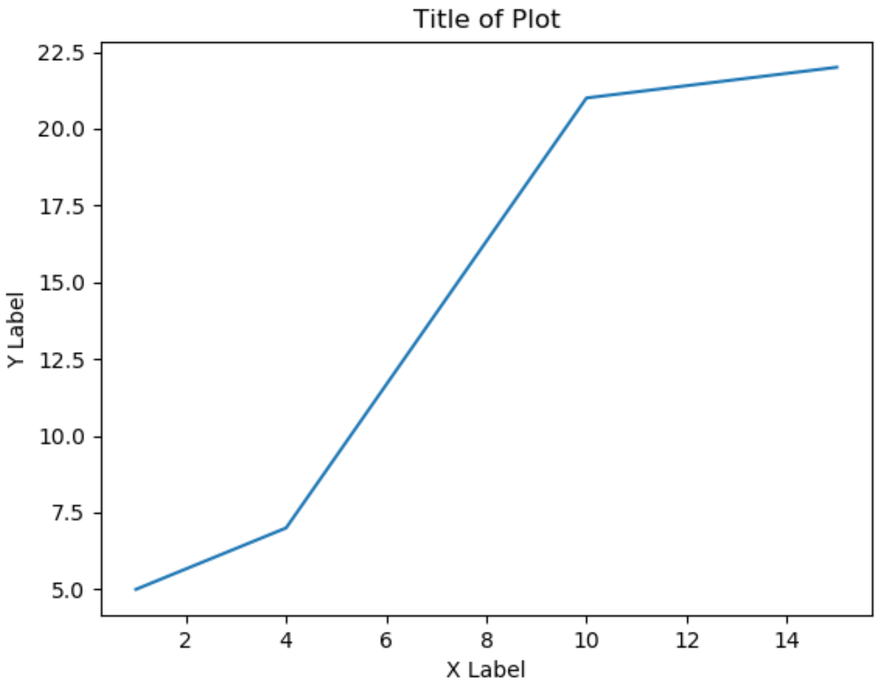
Следующий код показывает, как создать линейный график в Matplotlib и сохранить график с прозрачным фоном:

import matplotlib.pyplot as plt #define x and y x = [1, 4, 10, 15] y = [5, 7, 21, 22] #create line plot plt.plot (x, y) #add title and axis labels plt.title('Title of Plot') plt.xlabel('X Label') plt.ylabel('Y Label') #save plot with transparent background plt.savefig('my_plot.png', transparent= True ) 

Если я перейду к месту на своем компьютере, где сохранено изображение, я смогу его просмотреть:

Однако это плохо иллюстрирует прозрачный фон.

Для этого я могу поместить изображение на цветной фон в Excel:

Обратите внимание, что фон полностью прозрачен.

Вы можете сравнить это с точно таким же изображением, сохраненным без использования прозрачного аргумента:

#save plot without specifying transparent background plt.savefig('my_plot2.png') 

Фон белый, это цвет фона по умолчанию в Matplotlib.

Примечание.Полную онлайн-документацию по функции savefig() можно найти здесь .

Дополнительные ресурсы

В следующих руководствах объясняется, как выполнять другие распространенные операции в Matplotlib:

Источник