Plotting roc curve in python

Как понять ROC-кривые с помощью Python

Если вы погуглите ROC curve machine learning, то Википедия выдаст вам такой ответ: Кривая рабочих характеристик приёмника, или ROC-кривая, представляет собой график функции, который иллюстрирует диагностические возможности системы двоичного классификатора при изменении её порога распознавания.

Ещё одно частое описание ROC-кривой: ROC-кривая отражает чувствительность модели к разным порогам классификации. Новичков эти определения могут сбить с толку. Попробуем разобраться и развить представление о ROC-кривых.

Что за чертовщина эта ROC-кривая?

Вариант, как понять ROC-кривую: она описывает взаимосвязь между чувствительностью модели (TPR, или true positives rate — доля истинно положительных примеров) и её специфичностью (описываемой в отношении долей ложноположительных результатов: 1-FPR).

Давайте разовьём эту концепцию. TPR, или чувствительность модели, является соотношением корректных классификаций положительного класса, разделённых на все положительные классы, доступные из набора данных:

FPR — доля ложноположительных примеров, false positives rate. Это соотношение между ложными срабатываниями (количество прогнозов, ошибочно отнесённых в положительные), и всеми доступными отрицательными классами. Математически:

Обобщая: вы сравниваете, как чувствительность модели меняется по отношению к ложно положительным долям на разных порогах отсечения. Модель опирается на порог отсечения, чтобы принимать решения по входным данным и относить их к положительным.

Разделение проблемы с порогами отсечения

Поначалу интуиция толкала к пониманию роли порогов отсечения. Мне помогла мысленная картина:

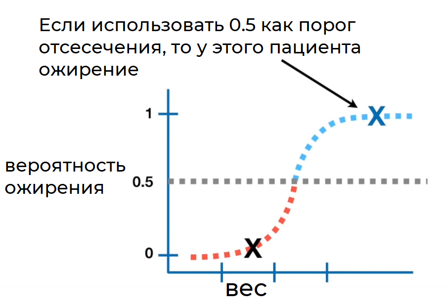
С такой классической визуализацией до меня дошло первое представление, а именно: идеальная модель — та, в которой доля истинно положительных результатов максимально высока, в то же время доля ложно положительных результатов удерживается как можно ниже.

Порог соответствует переменной T (например, значение между 0 и 1), служит границей принятия решения для классификатора и влияет на компромисс между TPR и FPR. Давайте напишем код, чтобы визуализировать все компоненты.

Визуализация ROC-кривой

1. Импортировать зависимости
2. Сгенерировать данные с помощью drawdata для Jupyter
3. Импортировать сгенерированные данные в фреймворк pandas
4. Подобрать модель логистической регрессии к данным
5. Получить прогнозы модели логистической регрессии в виде значений вероятности
6. Установить другие пороги отсечения
7. Визуализировать ROC-кривую
8. Сделать окончательные выводы

Импортируем зависимости

from drawdata import draw_scatter import pandas as pd from sklearn.model_selection import train_test_split from sklearn.linear_model import LogisticRegression from sklearn.metrics import accuracy_score, precision_recall_curve,precision_score, plot_roc_curve

Сгенерируем данные с помощью пакета drawdata для блокнотов Jupyter

Импортируем данные в фреймворк pandas

Подберём модель логистической регрессии к данным

def get_fp_tp(y, proba, threshold): """Возвращает количество долей ложно положительных и истинно положительных.""" # источник: https://towardsdatascience.com/roc-curve-explained-50acab4f7bd8 # Разносим по классам pred = pd.Series(np.where(proba>=threshold, 1, 0), dtype='category') pred.cat.set_categories([0,1], inplace=True) # Создаём матрицу ошибок confusion_matrix = pred.groupby([y, pred]).size().unstack()\ .rename(columns=, index=) false_positives = confusion_matrix.loc['actual_0', 'pred_1'] true_positives = confusion_matrix.loc['actual_1', 'pred_1'] return false_positives, true_positives # train / test split на примере сгенерированного датасета X = df[["x", "y"]].values Y = df["z"].values X_train, X_test, y_train, y_test = train_test_split(X, Y, test_size=0.2, random_state=42) y_test = np.array([1 if p=="a" else 0 for p in y_test]) y_train = np.array([1 if p=="a" else 0 for p in y_train]) # создаём модель lgr = LogisticRegression() lgr.fit(X_train, y_train)

Получим прогнозы модели логистической регрессии в виде значений вероятности

y_hat = lgr.predict_proba(X_test)[:,1]

Установим другие пороговые значения

thresholds = np.linspace(0,1,100)

Визуализируем ROC-кривую

# defining fpr and tpr tpr = [] fpr = [] # определяем положительные и отрицательные positives = np.sum(y_test==1) negatives = np.sum(y_test==0) # перебираем пороговые значения и получаем количество ложно и истинно положительных результатов for th in thresholds: fp,tp = get_fp_tp(y_test, y_hat, th) tpr.append(tp/positives) fpr.append(fp/negatives) plt.plot([0, 1], [0, 1], linestyle='--', lw=2, color='r',label='Random', alpha=.8) plt.plot(fpr,tpr, label="ROC Curve",color="blue") plt.text(0.5, 0.5, "varying threshold scores (0-1)", rotation=0, size=12,ha="center", va="center",bbox=dict(boxstyle="rarrow")) plt.xlabel("False Positve Rate") plt.ylabel("True Positive Rate") plt.legend() plt.show()

Сделаем окончательные выводы

Изменяя порог, мы получили возрастающие значения как истинно положительных, так и ложно положительных долей. В хорошей модели порог отсечения ставит истинно положительные доли как можно ближе к 1, при этом сохраняя ложно положительные доли на самом нижнем из возможных уровней.

Как нам выбрать лучший порог?

Простой способ: выбрать тот порог, у которого максимальная сумма из истинно положительных и ложно отрицательных долей (1-FPR).

Другой критерий: простой выбор точки, ближайшей к левому верхнему углу ROC-кривой. Однако такой критерий подразумевает, что истинно положительный и истинно отрицательный показатели имеют одинаковый вес. В некоторых случаях, такая выборка не подходит, поскольку отрицательное влияние ложно положительных долей весомее, чем влияние истинно положительных.

Итоговые выводы о ROC-кривой

Я считаю, что в долгосрочной перспективе машинного обучения полезно потратить время на освоение оценочных показателей. В этой статье вы узнали:

• Базовое представление о том, как работают ROC-кривые
• Как пороги отсечения влияют на соотношение чувствительности и особенности модели
• Как использовать ROC-кривые для выбора оптимальных порогов отсечения

Источник

sklearn.metrics .roc_curve¶

Note: this implementation is restricted to the binary classification task.

Parameters : y_true array-like of shape (n_samples,)

True binary labels. If labels are not either or , then pos_label should be explicitly given.

y_score array-like of shape (n_samples,)

Target scores, can either be probability estimates of the positive class, confidence values, or non-thresholded measure of decisions (as returned by “decision_function” on some classifiers).

pos_label int, float, bool or str, default=None

The label of the positive class. When pos_label=None , if y_true is in or , pos_label is set to 1, otherwise an error will be raised.

sample_weight array-like of shape (n_samples,), default=None

drop_intermediate bool, default=True

Whether to drop some suboptimal thresholds which would not appear on a plotted ROC curve. This is useful in order to create lighter ROC curves.

New in version 0.17: parameter drop_intermediate.

Increasing false positive rates such that element i is the false positive rate of predictions with score >= thresholds[i] .

tpr ndarray of shape (>2,)

Increasing true positive rates such that element i is the true positive rate of predictions with score >= thresholds[i] .

thresholds ndarray of shape (n_thresholds,)

Decreasing thresholds on the decision function used to compute fpr and tpr. thresholds[0] represents no instances being predicted and is arbitrarily set to np.inf .

Plot Receiver Operating Characteristic (ROC) curve given an estimator and some data.

Plot Receiver Operating Characteristic (ROC) curve given the true and predicted values.

Compute error rates for different probability thresholds.

Compute the area under the ROC curve.

Since the thresholds are sorted from low to high values, they are reversed upon returning them to ensure they correspond to both fpr and tpr , which are sorted in reversed order during their calculation.

An arbitrary threshold is added for the case tpr=0 and fpr=0 to ensure that the curve starts at (0, 0) . This threshold corresponds to the np.inf .

Fawcett T. An introduction to ROC analysis[J]. Pattern Recognition Letters, 2006, 27(8):861-874.

>>> import numpy as np >>> from sklearn import metrics >>> y = np.array([1, 1, 2, 2]) >>> scores = np.array([0.1, 0.4, 0.35, 0.8]) >>> fpr, tpr, thresholds = metrics.roc_curve(y, scores, pos_label=2) >>> fpr array([0. , 0. , 0.5, 0.5, 1. ]) >>> tpr array([0. , 0.5, 0.5, 1. , 1. ]) >>> thresholds array([ inf, 0.8 , 0.4 , 0.35, 0.1 ]) 

Источник

ROC Curve with Visualization API¶

Scikit-learn defines a simple API for creating visualizations for machine learning. The key features of this API is to allow for quick plotting and visual adjustments without recalculation. In this example, we will demonstrate how to use the visualization API by comparing ROC curves.

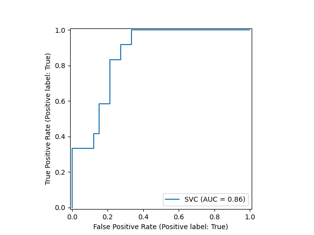
Load Data and Train a SVC¶

First, we load the wine dataset and convert it to a binary classification problem. Then, we train a support vector classifier on a training dataset.

import matplotlib.pyplot as plt from sklearn.datasets import load_wine from sklearn.ensemble import RandomForestClassifier from sklearn.metrics import RocCurveDisplay from sklearn.model_selection import train_test_split from sklearn.svm import SVC X, y = load_wine(return_X_y=True) y = y == 2 X_train, X_test, y_train, y_test = train_test_split(X, y, random_state=42) svc = SVC(random_state=42) svc.fit(X_train, y_train) 

In a Jupyter environment, please rerun this cell to show the HTML representation or trust the notebook.
On GitHub, the HTML representation is unable to render, please try loading this page with nbviewer.org.

Plotting the ROC Curve¶

Next, we plot the ROC curve with a single call to sklearn.metrics.RocCurveDisplay.from_estimator . The returned svc_disp object allows us to continue using the already computed ROC curve for the SVC in future plots.

svc_disp = RocCurveDisplay.from_estimator(svc, X_test, y_test) plt.show() 

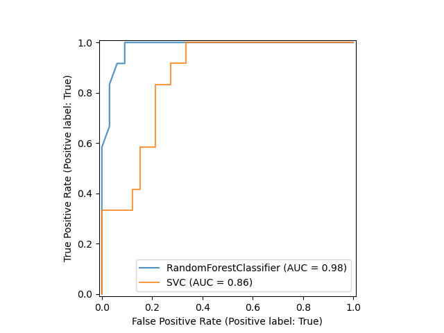
Training a Random Forest and Plotting the ROC Curve¶

We train a random forest classifier and create a plot comparing it to the SVC ROC curve. Notice how svc_disp uses plot to plot the SVC ROC curve without recomputing the values of the roc curve itself. Furthermore, we pass alpha=0.8 to the plot functions to adjust the alpha values of the curves.

rfc = RandomForestClassifier(n_estimators=10, random_state=42) rfc.fit(X_train, y_train) ax = plt.gca() rfc_disp = RocCurveDisplay.from_estimator(rfc, X_test, y_test, ax=ax, alpha=0.8) svc_disp.plot(ax=ax, alpha=0.8) plt.show() 

Total running time of the script: ( 0 minutes 0.157 seconds)

Источник