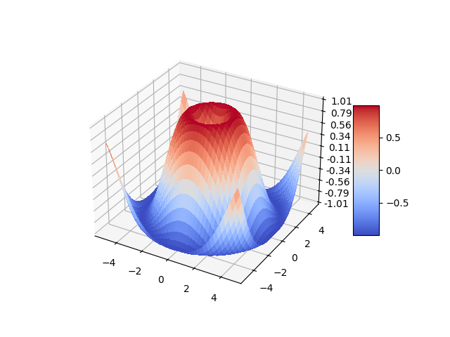
- 3D surface (colormap)#
- The mplot3d toolkit#
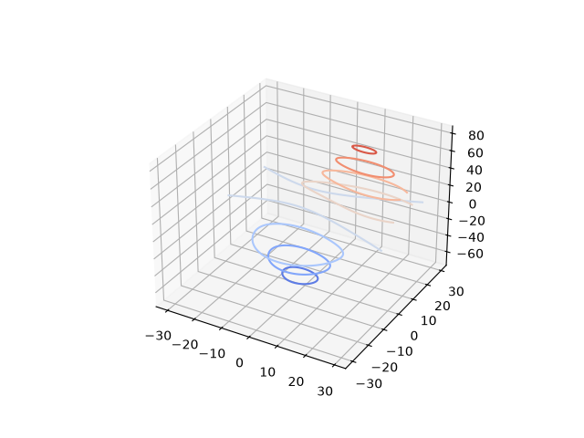
- Line plots#
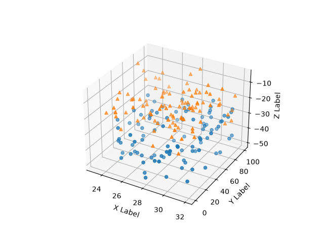
- Scatter plots#
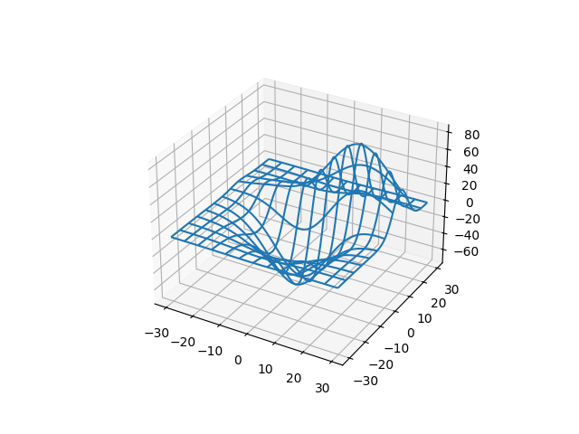
- Wireframe plots#
- Surface plots#
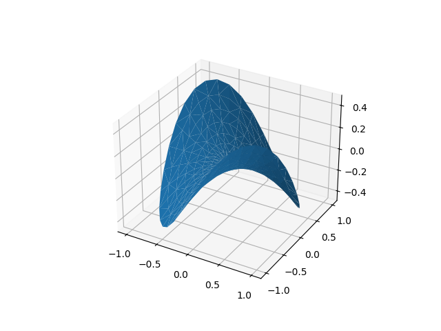
- Tri-Surface plots#
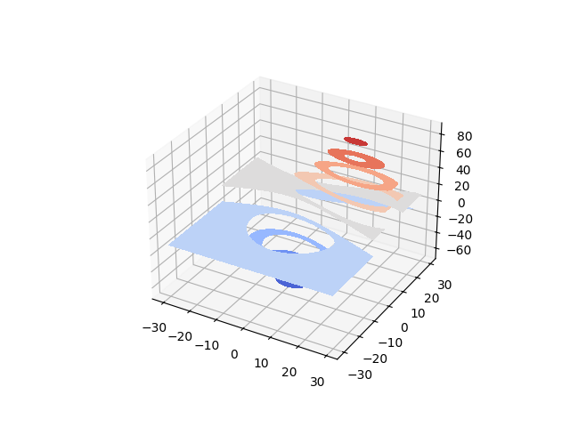
- Contour plots#
- Filled contour plots#
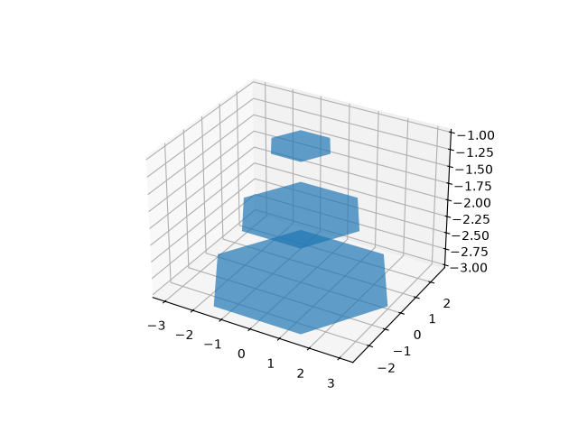
- Polygon plots#
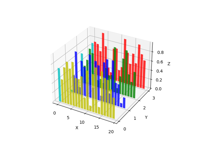
- Bar plots#
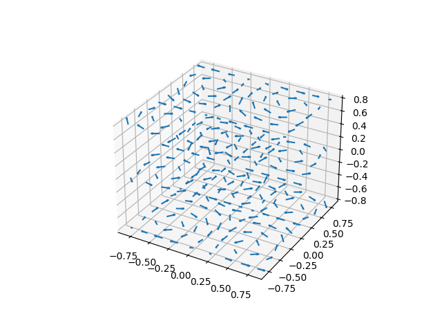
- Quiver#
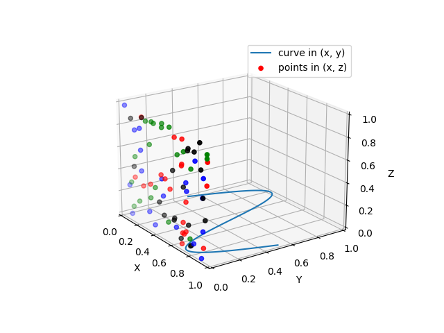
- 2D plots in 3D#
- Text#
- Matplotlib 3D Surface Plot — plot_surface() Function
- Creation of 3D Surface Plot
- plot_surface() Attributes
- 3D Surface Plot Basic Example
- Gradient Surface Plot
- Gradient Surface Plot Example
- Matplotlib. Урок 5. Построение 3D графиков. Работа с mplot3d Toolkit
- Линейный график
- Точечный график
- Каркасная поверхность
- Поверхность
- P.S.
- Matplotlib. Урок 5. Построение 3D графиков. Работа с mplot3d Toolkit : 2 комментария
3D surface (colormap)#
Demonstrates plotting a 3D surface colored with the coolwarm colormap. The surface is made opaque by using antialiased=False .
Also demonstrates using the LinearLocator and custom formatting for the z axis tick labels.
import matplotlib.pyplot as plt from matplotlib import cm from matplotlib.ticker import LinearLocator import numpy as np fig, ax = plt.subplots(subplot_kw="projection": "3d">) # Make data. X = np.arange(-5, 5, 0.25) Y = np.arange(-5, 5, 0.25) X, Y = np.meshgrid(X, Y) R = np.sqrt(X**2 + Y**2) Z = np.sin(R) # Plot the surface. surf = ax.plot_surface(X, Y, Z, cmap=cm.coolwarm, linewidth=0, antialiased=False) # Customize the z axis. ax.set_zlim(-1.01, 1.01) ax.zaxis.set_major_locator(LinearLocator(10)) # A StrMethodFormatter is used automatically ax.zaxis.set_major_formatter(' ') # Add a color bar which maps values to colors. fig.colorbar(surf, shrink=0.5, aspect=5) plt.show()

The use of the following functions, methods, classes and modules is shown in this example:
The mplot3d toolkit#
This tutorial showcases various 3D plots. Click on the figures to see each full gallery example with the code that generates the figures.
3D Axes (of class Axes3D ) are created by passing the projection=»3d» keyword argument to Figure.add_subplot :
import matplotlib.pyplot as plt fig = plt.figure() ax = fig.add_subplot(projection='3d')
Multiple 3D subplots can be added on the same figure, as for 2D subplots.
Changed in version 3.2.0: Prior to Matplotlib 3.2.0, it was necessary to explicitly import the mpl_toolkits.mplot3d module to make the ‘3d’ projection to Figure.add_subplot .
See the mplot3d FAQ for more information about the mplot3d toolkit.
Line plots#
See Axes3D.plot for API documentation.
Scatter plots#
See Axes3D.scatter for API documentation.
Wireframe plots#
See Axes3D.plot_wireframe for API documentation.
Surface plots#
See Axes3D.plot_surface for API documentation.
Tri-Surface plots#
See Axes3D.plot_trisurf for API documentation.
Contour plots#
See Axes3D.contour for API documentation.
Filled contour plots#
See Axes3D.contourf for API documentation.
New in version 1.1.0: The feature demoed in the second contourf3d example was enabled as a result of a bugfix for version 1.1.0.
Polygon plots#
Bar plots#
See Axes3D.bar for API documentation.
Quiver#
See Axes3D.quiver for API documentation.
2D plots in 3D#
Text#
See Axes3D.text for API documentation.
Matplotlib 3D Surface Plot — plot_surface() Function
In this tutorial, we will cover how to create a 3D Surface Plot in the matplotlib library.
In Matplotlib’s mpl_toolkits.mplot3d toolkit there is axes3d present that provides the necessary functions that are very useful in creating 3D surface plots.
The representation of a three-dimensional dataset is mainly termed as the Surface Plot.
- One thing is important to note that the surface plot provides a relationship between two independent variables that are X and Z and a designated dependent variable that is Y, rather than just showing the individual data points.
- The Surface plot is a companion plot to the Contour Plot and it is similar to wireframe plot but there is a difference too and it is each wireframe is basically a filled polygon.
- With the help of this, the topology of the surface can be visualized very easily.
Creation of 3D Surface Plot
To create the 3-dimensional surface plot the ax.plot_surface() function is used in matplotlib.
The required syntax for this function is given below:
In the above syntax, the X and Y mainly indicate a 2D array of points x and y while Z is used to indicate the 2D array of heights.
plot_surface() Attributes
Some attributes of this function are as given below:
This attribute is used to shade the face color.
2. facecolors
This attribute is used to indicate the face color of the individual surface
This attribute indicates the maximum value of the map.
This attribute indicates the minimum value of the map.
This attribute acts as an instance to normalize the values of color map
This attribute indicates the color of the surface
This attribute indicates the colormap of the surface
This attribute is used to indicate the number of rows to be used The default value of this attribute is 50
This attribute is used to indicate the number of columns to be used The default value of this attribute is 50
This attribute is used to indicate the array of row stride(that is step size)
This attribute is used to indicate the array of column stride(that is step size)
3D Surface Plot Basic Example
Below we have a code where we will use the above-mentioned function to create a 3D Surface Plot:
from mpl_toolkits import mplot3d import numpy as np import matplotlib.pyplot as plt x = np.outer(np.linspace(-4, 4, 33), np.ones(33)) y = x.copy().T z = (np.sin(x **2) + np.cos(y **2) ) fig = plt.figure(figsize =(14, 9)) ax = plt.axes(projection ='3d') ax.plot_surface(x, y, z) plt.show() The output for the above code is as follows:

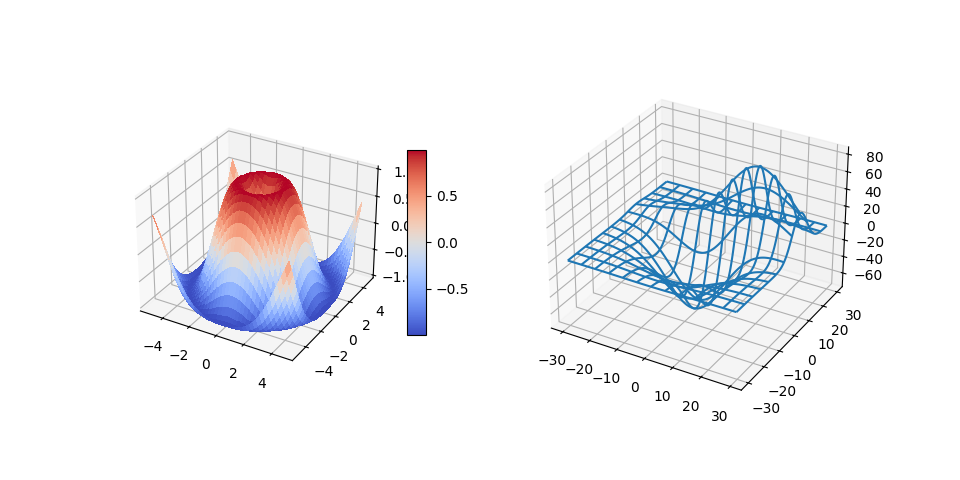
Gradient Surface Plot
This plot is a combination of a 3D surface plot with a 2D contour plot. In the Gradient surface plot, the 3D surface is colored same as the 2D contour plot. The parts that are high on the surface contains different color rather than the parts which are low at the surface.
ax.plot_surface(X, Y, Z, cmap, linewidth, antialiased)where cmap is used to set the color for the surface.
Gradient Surface Plot Example
Now it’s time to cover a gradient surface plot. The code snippet for the same is given below:
from mpl_toolkits import mplot3d import numpy as np import matplotlib.pyplot as plt x = np.outer(np.linspace(-3, 3, 32), np.ones(32)) y = x.copy().T z = (np.sin(x **2) + np.cos(y **2) ) fig = plt.figure(figsize =(14, 9)) ax = plt.axes(projection ='3d') my_cmap = plt.get_cmap('cool') surf = ax.plot_surface(x, y, z, cmap = my_cmap, edgecolor ='none') fig.colorbar(surf, ax = ax, shrink = 0.7, aspect = 7) ax.set_title('Surface plot') plt.show() The output for the above code is as follows:

Matplotlib. Урок 5. Построение 3D графиков. Работа с mplot3d Toolkit


До этого момента все графики, которые мы строили были двумерные, Matplotlib позволяет строить 3D графики. Этой теме посвящен данный урок.
Импортируем необходимые модули для работы с 3D :
import matplotlib.pyplot as plt from mpl_toolkits.mplot3d import Axes3D
В библиотеке доступны инструменты для построения различных типов графиков. Рассмотрим некоторые из них более подробно.
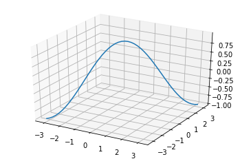
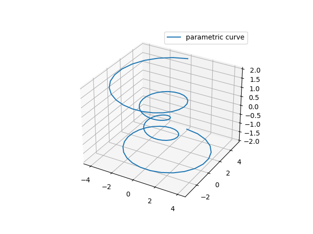
Линейный график
Для построения линейного графика используется функция plot().
Axes3D.plot(self, xs, ys, *args, zdir=’z’, **kwargs)
- xs : 1D массив
- x координаты.
- y координаты.
- z координаты. Если передан скаляр, то он будет присвоен всем точкам графика.
- Определяет ось, которая будет принята за z направление, значение по умолчанию: ‘z’ .
- Дополнительные аргументы, аналогичные тем, что используются в функции plot() для построения двумерных графиков.
x = np.linspace(-np.pi, np.pi, 50) y = x z = np.cos(x) fig = plt.figure() ax = fig.add_subplot(111, projection='3d') ax.plot(x, y, z, label='parametric curve')

Точечный график
Для построения точечного графика используется функция scatter() .
Axes3D.scatter(self, xs, ys, zs=0, zdir=’z’, s=20, c=None, depthshade=True, *args, **kwargs)
- xs, ys : массив
- Координаты точек по осям x и y .
- Координаты точек по оси z . Если передан скаляр, то он будет присвоен всем точкам графика. Значение по умолчанию: 0.
- Определяет ось, которая будет принята за z направление, значение по умолчанию: ‘z’
- Размер маркера. Значение по умолчанию: 20.
- Цвет маркера. Возможные значения:
- Строковое значение цвета для всех маркеров.
- Массив строковых значений цвета.
- Массив чисел, которые могут быть отображены в цвета через функции cmap и norm .
- 2D массив, элементами которого являются RGB или RGBA .
- Затенение маркеров для придания эффекта глубины.
- Дополнительные аргументы, аналогичные тем, что используются в функции scatter() для построения двумерных графиков.
np.random.seed(123) x = np.random.randint(-5, 5, 40) y = np.random.randint(0, 10, 40) z = np.random.randint(-5, 5, 40) s = np.random.randint(10, 100, 20) fig = plt.figure() ax = fig.add_subplot(111, projection='3d') ax.scatter(x, y, z, s=s)
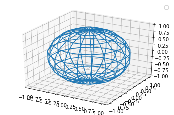
Каркасная поверхность
Для построения каркасной поверхности используется функция plot_wireframe() .
plot_wireframe(self, X, Y, Z, *args, **kwargs)
- X, Y, Z: 2D массивы
- Данные для построения поверхности.
- Максимальное количество элементов каркаса, которое будет использовано в каждом из направлений. Значение по умолчанию: 50.
- Параметры определяют величину шага, с которым будут браться элементы строки / столбца из переданных массивов. Параметры rstride , cstride и rcount , ccount являются взаимоисключающими.
- Дополнительные аргументы, определяемые Line3DCollection .
u, v = np.mgrid[0:2*np.pi:20j, 0:np.pi:10j] x = np.cos(u)*np.sin(v) y = np.sin(u)*np.sin(v) z = np.cos(v) fig = plt.figure() ax = fig.add_subplot(111, projection='3d') ax.plot_wireframe(x, y, z) ax.legend()
Поверхность
Для построения поверхности используйте функцию plot_surface().
plot_surface(self, X, Y, Z, *args, norm=None, vmin=None, vmax=None, lightsource=None, **kwargs)
- X, Y, Z : 2D массивы
- Данные для построения поверхности.
- см. rcount , ccount в “Каркасная поверхность“.
- см. rstride , cstride в “Каркасная поверхность“.
- Цвет для элементов поверхности.
- Colormap для элементов поверхности.
- Индивидуальный цвет для каждого элемента поверхности.
- Нормализация для colormap .
- Границы нормализации.
- Использование тени для facecolors . Значение по умолчанию: True.
- Объект класса LightSource – определяет источник света, используется, только если shade = True .
- Дополнительные аргументы, определяемые Poly3DCollection .
u, v = np.mgrid[0:2*np.pi:20j, 0:np.pi:10j] x = np.cos(u)*np.sin(v) y = np.sin(u)*np.sin(v) z = np.cos(v) fig = plt.figure() ax = fig.add_subplot(111, projection='3d') ax.plot_surface(x, y, z, cmap='inferno') ax.legend()
P.S.
Вводные уроки по “Линейной алгебре на Python” вы можете найти соответствующей странице нашего сайта . Все уроки по этой теме собраны в книге “Линейная алгебра на Python”.
Если вам интересна тема анализа данных, то мы рекомендуем ознакомиться с библиотекой Pandas. Для начала вы можете познакомиться с вводными уроками. Все уроки по библиотеке Pandas собраны в книге “Pandas. Работа с данными”.
Matplotlib. Урок 5. Построение 3D графиков. Работа с mplot3d Toolkit : 2 комментария