matplotlib.pyplot.bar#
The bars are positioned at x with the given alignment. Their dimensions are given by height and width. The vertical baseline is bottom (default 0).
Many parameters can take either a single value applying to all bars or a sequence of values, one for each bar.
Parameters : x float or array-like
The x coordinates of the bars. See also align for the alignment of the bars to the coordinates.
height float or array-like
width float or array-like, default: 0.8
bottom float or array-like, default: 0
The y coordinate(s) of the bottom side(s) of the bars.
align , default: ‘center’
Alignment of the bars to the x coordinates:
- ‘center’: Center the base on the x positions.
- ‘edge’: Align the left edges of the bars with the x positions.
To align the bars on the right edge pass a negative width and align=’edge’ .
Container with all the bars and optionally errorbars.
Other Parameters : color color or list of color, optional
The colors of the bar faces.
edgecolor color or list of color, optional
The colors of the bar edges.
linewidth float or array-like, optional
Width of the bar edge(s). If 0, don’t draw edges.
tick_label str or list of str, optional
The tick labels of the bars. Default: None (Use default numeric labels.)
label str or list of str, optional
A single label is attached to the resulting BarContainer as a label for the whole dataset. If a list is provided, it must be the same length as x and labels the individual bars. Repeated labels are not de-duplicated and will cause repeated label entries, so this is best used when bars also differ in style (e.g., by passing a list to color.)
xerr, yerr float or array-like of shape(N,) or shape(2, N), optional
If not None, add horizontal / vertical errorbars to the bar tips. The values are +/- sizes relative to the data:
- scalar: symmetric +/- values for all bars
- shape(N,): symmetric +/- values for each bar
- shape(2, N): Separate — and + values for each bar. First row contains the lower errors, the second row contains the upper errors.
- None: No errorbar. (Default)
See Different ways of specifying error bars for an example on the usage of xerr and yerr.
ecolor color or list of color, default: ‘black’
The line color of the errorbars.
capsize float, default: rcParams[«errorbar.capsize»] (default: 0.0 )
The length of the error bar caps in points.
error_kw dict, optional
Dictionary of keyword arguments to be passed to the errorbar method. Values of ecolor or capsize defined here take precedence over the independent keyword arguments.
log bool, default: False
If True, set the y-axis to be log scale.
data indexable object, optional
If given, all parameters also accept a string s , which is interpreted as data[s] (unless this raises an exception).
a filter function, which takes a (m, n, 3) float array and a dpi value, and returns a (m, n, 3) array and two offsets from the bottom left corner of the image
Рисуем гистограммы, столбчатые и круговые диаграммы
На этом занятии мы продолжим знакомство с разными типами двумерных графиков и увидим, как можно строить столбчатые и круговые диаграммы.
Гистограмма и столбчатые диаграммы
Иногда данные требуется сгруппировать по определенным диапазонам и подсчитать сколько значений попадает в тот или иной интервал. Для выполнения такой задачи хорошо подходят столбчатые диаграммы и довольно известный их вид – это гистограмма распределения случайной величины.
Давайте сгенерируем вектор из 500 случайных величин и выведем их в виде гистограммы, используя функцию hist():
import numpy as np import matplotlib.pyplot as plt fig = plt.figure(figsize=(6, 4)) ax = fig.add_subplot() y = np.random.normal(0, 2, 500) ax.hist(y) ax.grid() plt.show()
На выходе получим следующее изображение распределения нормальной СВ:

Фактически, мы здесь имеем набор столбиков, высота которых определяется числом СВ, попавших в тот или иной диапазон. Причем, по умолчанию функция hist() разбивает весь интервал на равных 10 диапазонов. Если требуется изменить это число, то мы можем его указать вторым параметром:
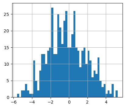
Прежний интервал теперь разбит на 50 диапазонов, столбиков стало больше и они выглядят тоньше.
Функции bar() и barh()
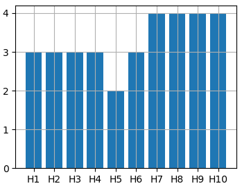
Похожий график можно сформировать и с помощью функции bar. Ей на вход, в самом простом варианте, нужно передать список отметок для столбцов x и значения высот каждого столбца y:
x = [f'H' for i in range(10)] y = np.random.randint(1, 5, len(x)) ax.bar(x, y)
Или, можно отобразить то же распределение нормальной СВ с помощью такой столбчатой диаграммы. Сначала сформируем сами величины и разобьем весь интервал на 10 равных диапазонов:
y = np.random.normal(0, 2, 500) x = np.linspace(np.min(y), np.max(y), 10)
Затем, подсчитаем, сколько величин попало в соответствующий диапазон и выведем список bars с помощью функции bar():
bars = [len(y[np.bitwise_and(y >= x[i], y x[i+1])]) for i in range(len(x)-1)] ax.bar(range(len(x)-1), bars)
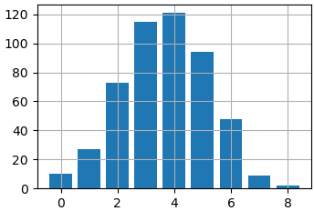
Как видите, у нас получилось изображение аналогичное гистограмме. Только пришлось предварительно подготовить данные, что не очень удобно. Поэтому, когда нужно вывести распределение величин по диапазонам, то проще использовать функцию hist().
Если нам нужно отображать столбики относительно оси ординат, то для этого существует функция barh(), которая работает аналогично функции bar():
В итоге, график будет выглядеть, следующим образом: