Pid controller in python

How to use Python for PID controller design

When I was in the university, my control system classes was dictated using MATLAB, MATLAB is a powerfull tool to design and test control systems. But, one of the things that overwhelms me about Matlab, is that it is a very heavy program with different types of packages for different uses and a large number of tools and I like a simple minimalist coding style stuff for create or design controllers.

As I am familiar with Python, I became curious to utilize this language to design a basic control system such as a PID controller, applying the theory I learned in university.

So here is what I learned.

What is a PID controller?

A PID controller is a «brain» for machines that helps them stay on track. It takes in sensory input, compares it to a target, and adjusts as needed to achieve the desired outcome.

A basic diagram of a PID controller looks like this:

e(t) is known as the error signal, which is the difference between a desired process value or setpoint r(t) and a measured process variable y(t) from the system that we want to control called «plant». u(t) is the output of the PID controller known as the control signal that will attempts to minimize the error e(t) over time.

The PID controller is made up of three distinct parts: the proportional component, the integral component, and the derivative component.

The proportional part helps to maintain the desired output of the control system by working to reduce the difference between the desired output and the actual output of the system. For example, the cruise control that keeps you at the right speed when you’re driving on a flat road. If you start going too slow, the proportional part tells the car to go a little faster so you get back to the right speed. If you start going too fast, it tells the car to go slower.

The integral part, keeps track of how much the system has been off from the desired output in the past and makes adjustments to help reduce that difference over time. It’s like a person who remembers that they were too hot or too cold in a room yesterday and adjusts the thermostat today to make sure they’re more comfortable.

The derivative part of a PID controller is like a watchdog that watches how things are changing over time. It looks for how fast things are changing and makes adjustments based on that. Imagine you’re going downhill in your car and you start going faster, the derivative part of a cruise control system would sense this change in speed and make adjustments to slow you down.

Mathematically, in time domain the PID controller looks like this:

u ( t ) = K p e ( t ) + K i ∫ 0 t e ( τ ) d τ + K d d d t e ( t ) u(t) = K_p e(t) + K_i \int_<0>^ e(\tau) d\tau + K_d \frac e(t) u ( t ) = K p ​ e ( t ) + K i ​ ∫ 0 t ​ e ( τ ) d τ + K d ​ d t d ​ e ( t )

• K p K_p K p ​ : represents how much the output of the controller changes in response to a difference between the desired output and the actual output of the system.
• K i K_i K i ​ : represents how much the output of the controller changes in response to the accumulated difference between the desired and actual outputs of the system over time.
• K d K_d K d ​ : represents how much the output of the controller changes in response to the rate of change of the difference between the desired and actual outputs of the system.
• e ( t ) e(t) e ( t ) : represents the error signal.
• u ( t ) u(t) u ( t ) : represents control signal.

Desiging the PID controller

We will be using example 8-1 (found on page 572) from the book ‘Modern Control Engineering’ by Katushiko Ogata to create our PID controller. Additionally, we will utilize the python-control library, as well as sympy and numpy for mathematical operations, and Matplotlib for visualizing the controller’s responses.

Creating the Plant model

We need a system plant to control before creating our PID controller. To do this, we can utilize the python-control package.

You might be curious as to why ‘s’ is used instead of time in the Laplace domain. The reason is that the Laplace domain enables analysis of transfer functions in a simpler and more efficient manner for linear time-invariant systems (LTI)

So we create our model transfer function system like this.

import control s = control.TransferFunction.s plant = 1/(s*(s+1)*(s+5)) 

Creating the PID model

Let’s create our PID in Laplace domain.

G c ( s ) = K p ( 1 + 1 T i s + T d s ) G_(s) = K_

(1 + \fracs> + T_s) G c ​ ( s ) = K p ​ ( 1 + T i ​ s 1 ​ + T d ​ s )

• K p K_

  K p ​ : represents how much the output of the controller changes in response to a difference between the desired output and the actual output of the system.

• T i T_ T i ​ : represents the integral time.
• T d T_ T d ​ : represents the derivative time.

Our goal now is to adjust the values of K p K_

K p ​ , T i T_ T i ​ , and T d T_ T d ​ for optimal performance. We will utilize the Ziegler-Nichols tuning rule to determine these values.

Since our plant contains an integrator ( 1 / s 1/s 1/ s ), we will utilize the second method of the Ziegler-Nichols tuning rule. This involves setting T i = ∞ Ti = \infty T i = ∞ cancelling it’s effect and T d = 0 Td = 0 T d = 0 in order to obtain the closed-loop transfer function.

Having obtained the transfer function of our plant using python-control, we can employ the feedback method to determine the closed-loop transfer function. To calculate this, we will add an arbitrary value to K p K_

K p ​ , set T d T_ T d ​ to 0, and assign a large value to T i T_ T i ​ .

import control s = control.TransferFunction.s plant = 1/(s*(s+1)*(s+5)) Kp = 17 Ti = 10000000000 Td = 0 pid = Kp*(1 + 1/Ti*s + Td*s) feedback = control.feedback(plant*pid) print(feedback) #result # 1.7e-08 s + 17 #---------------------- #s^3 + 6 s^2 + 5 s + 17 

If you look at the numerator, you will notice it has a term of 1.7 e − 08 s + 17 1.7e-08s + 17 1.7 e − 08 s + 17 . The value 17 corresponds to our parameter K p K_

K p ​ , while the value 1.7 e − 08 s 1.7e-08s 1.7 e − 08 s is practically negligible. As a result, we can consider our closed-loop transfer function to be:

Y ( s ) R ( s ) = K p s 3 + 6 s 2 + 5 s + K p \frac = \frac> + 6s^ + 5s + K_

> R ( s ) Y ( s ) ​ = s 3 + 6 s 2 + 5 s + K p ​ K p ​ ​

Where s 3 + 6 s 2 + 5 s + K p = 0 s^ + 6s^ + 5s + K_

= 0 s 3 + 6 s 2 + 5 s + K p ​ = 0 will be our charateristic equation.

Our next step involves determining a value for K p K_

K p ​ that will render the plant marginally stable, thereby promoting sustained oscillation. This can be achieved using Routh’s stability criterion. In Python, we can leverage the method outlined in the tbcontrol library to accomplish this.

def routh(p): coefficients = p.all_coeffs() N = len(coefficients) M = sympy.zeros(N, (N+1)//2 + 1) r1 = coefficients[0::2] r2 = coefficients[1::2] M[0, :len(r1)] = [r1] M[1, :len(r2)] = [r2] for i in range(2, N): for j in range(N//2): S = M[[i-2, i-1], [0, j+1]] M[i, j] = sympy.simplify(-S.det()/M[i-1,0]) return M[:, :-1] 

Then we can implement it like this:

import sympy Kp = sympy.Symbol('Kp') s = sympy.Symbol('s') ce = s**3 + 6*s**2 + 5*s + Kp #charateristic equation A = routh(sympy.Poly(ce,s)) A 

[ 1 5 6 K p 5 − K p 6 0 K p 0 ] \begin 1 & 5\\ 6 & K_

\\ 5-\frac> & 0\\ K_

& 0 \end

​ 1 6 5 − 6 K p ​ ​ K p ​ ​ 5 K p ​ 0 0 ​

To check the stability limits we can use sympy like this.

sympy.solve([e > 0 for e in A[:,0]], Kp) 

We have determined that the critical K p K_

K p ​ value is 30, which represents the threshold for sustaining oscillation. Accordingly, the critical gain can be expressed as K c r = 30 K_ = 30 K cr ​ = 30 . With this value in place, the characteristic equation takes on the following form:

To find the frequency of the sustained oscillation, we replace s = j w s=jw s = j w getting.

( j ω ) 3 + 6 ( j ω ) 2 + 5 ( j ω ) + 30 = 0 (j\omega)^ <3>+ 6(j\omega)^ + 5(j\omega) + 30 = 0 ( jω ) 3 + 6 ( jω ) 2 + 5 ( jω ) + 30 = 0

6 ( 5 − ω 2 ) + j ω ( 5 − ω 2 ) = 0 6(5-\omega^<2>) + j\omega(5-\omega^<2>) = 0 6 ( 5 − ω 2 ) + jω ( 5 − ω 2 ) = 0

where the frequency of the sustained oscillation will be

ω 2 = 5 = > ω = 5 \omega^ = 5 => \omega = \sqrt ω 2 = 5 => ω = 5

We can also solve this directly using sympy like this.

s = sympy.Symbol('s') ce = s**3 + 6*s**2 + 5*s + 30 roots = sympy.solve(ce,s) roots 

Finally, using the Ziegler–Nichols Rule, we determine the values of K p , T i , T d K_

, T_, T_ K p ​ , T i ​ , T d ​

K p = 0.6 K c r T i = 0.5 P c r T d = 0.125 P c r \begin K_

= 0.6K_ \\ T_ = 0.5P_ \\ T_ = 0.125P_ \end K p ​ = 0.6 K cr ​ T i ​ = 0.5 P cr ​ T d ​ = 0.125 P cr ​ ​

Where P c r = 2 π ω P_ = \frac<2\pi> <\omega>P cr ​ = ω 2 π ​

import numpy as np w = np.sqrt(5) Pcr = (2*np.pi)/w Kcr = 30 Kp = 0.6*Kcr Ti = 0.5*Pcr Td = 0.125*Pcr print("Kp:", Kp) print("Ti:", Ti) print("Td:", Td) #result #Kp: 18.0 #Ti: 1.40496. #Td: 0.3512. 

Testing the PID

Now that we’ve tuned our PID controller, the next step is to evaluate the system’s behavior. One way to accomplish this is by plotting the step response using the python-control library. This can be achieved as follows:

s = control.TransferFunction.s plant = (1/(s*(s+1)*(s+5))) Kp = 18 Ti = 1.405 Td = 0.351 pid = (Kp*(1 + 1/(Ti*s) + Td*s)) feedback = control.feedback(system*pid) print(feedback) #result # 8.877 s^2 + 25.29 s + 18 #---------------------------------------------- #1.405 s^4 + 8.43 s^3 + 15.9 s^2 + 25.29 s + 18 t = np.linspace(0,17) T, y = control.step_response(feedback, t) # plot plt.plot(T, y) plt.xlabel('Time (seconds)') plt.ylabel('Output') plt.title('Step Response') plt.grid() plt.show()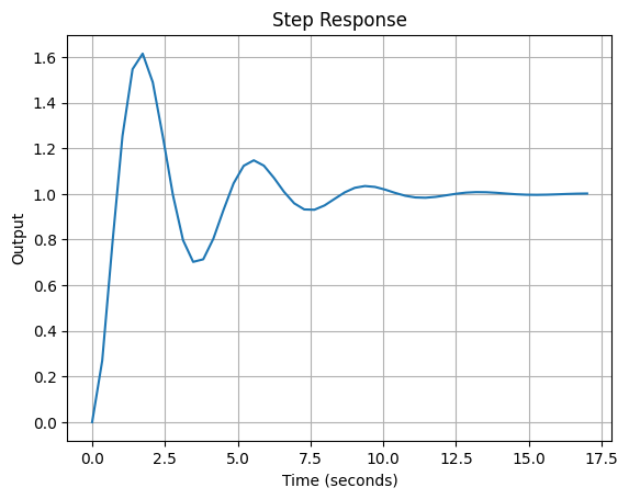 

You can also get specific information using the step_info method of python-control like the overshoot or RiseTime. etc.

info = control.step_info(feedback) print("feedback info") print("-------------") print("RiseTime:",info["RiseTime"]) print("Overshoot:", info["Overshoot"]) #result #feedback info #------------- #RiseTime: 0.5058786385507097 #Overshoot: 93.70305071110504 

So that’s all for now! You’ve seen how Python can be used to design a simple PID controller, using the Ziegler-Nichols method as one of many techniques to determine the PID parameters. Keep in mind that this approach may not always produce optimal values for your specific needs. From here, you can start experimenting with different techniques to fine-tune your controller using the libraries that we use.

You can check the full code here

I hope this has been helpful, and I’ll see you soon!

References

• [1] Katushiko Ogata.»Modern Control Engineering fifth Edition». Prentice Hall.
• [2] Carl Sandrock. «Dynamics and Control with jupyter notebooks».
• [3] Carl Sandrock. «tbcontrol library».
• [4] Python-control.org. «Python Control System Library».
• [5] Sympy Developer Team. Sympy Documentation.
• [6] PID Controller wikipedia.

Источник

Saved searches

Use saved searches to filter your results more quickly

You signed in with another tab or window. Reload to refresh your session. You signed out in another tab or window. Reload to refresh your session. You switched accounts on another tab or window. Reload to refresh your session.

A simple and easy to use PID controller in Python

License

m-lundberg/simple-pid

This commit does not belong to any branch on this repository, and may belong to a fork outside of the repository.

Name already in use

A tag already exists with the provided branch name. Many Git commands accept both tag and branch names, so creating this branch may cause unexpected behavior. Are you sure you want to create this branch?

Sign In Required

Please sign in to use Codespaces.

Launching GitHub Desktop

If nothing happens, download GitHub Desktop and try again.

Launching GitHub Desktop

If nothing happens, download GitHub Desktop and try again.

Launching Xcode

If nothing happens, download Xcode and try again.

Launching Visual Studio Code

Your codespace will open once ready.

There was a problem preparing your codespace, please try again.

Latest commit

Git stats

Files

Failed to load latest commit information.

README.md

A simple and easy to use PID controller in Python. If you want a PID controller without external dependencies that just works, this is for you! The PID was designed to be robust with help from Brett Beauregards guide.

from simple_pid import PID pid = PID(1, 0.1, 0.05, setpoint=1) # Assume we have a system we want to control in controlled_system v = controlled_system.update(0) while True: # Compute new output from the PID according to the systems current value control = pid(v) # Feed the PID output to the system and get its current value v = controlled_system.update(control)

python -m pip install simple-pid 

Documentation, including a user guide and complete API reference, can be found here.

This project has a test suite using pytest . To run the tests, install pytest and run:

Источник