Оператор матричного умножения python

Произведение матриц и векторов, элементы линейной алгебры

Пришло время познакомиться с одной из фундаментальных возможностей пакета NumPy–матричных и векторных вычислений. На одном из прошлых занятий мы с вами уже видели, как можно поэлементно умножать один вектор на другой или одну матрицу на другую:

a = np.arange(1, 10).reshape(3, 3) b = np.arange(10, 19).reshape(3, 3) a*b

В консоли увидим результат:

array([[ 10, 22, 36],
[ 52, 70, 90],
[112, 136, 162]])

Матричное умножение

Но если нам нужно выполнить именно матричное умножение, то есть, строки одной матрицы умножать на столбцы другой и результаты складывать:

то для этого следует использовать специальные функции и операторы. Начнем с функций. Итак, чтобы перемножить две матрицы a иbпо всем правилам математики, запишем следующую команду:

Эта функция возвращает новую матрицу (двумерный массив) с результатом умножения:

array([[ 84, 90, 96],
[201, 216, 231],
[318, 342, 366]])

Тот же результат можно получить и с помощью функции:

Считается, что этот вариант предпочтительнее использовать при умножении матриц.

Векторное умножение

Аналогичные операции можно выполнять и с векторами. Математически, если у нас имеются два вектора:

то их умножение можно реализовать в двух видах:

Первое умножение реализуется либо через функцию:

a = np.arange(1, 10) b = np.ones(9) np.dot(a, b) # значение 45

Либо, более предпочтительной функцией для внутреннего умножения векторов:

Второй вариант умножения (внешнее умножение векторов) реализуется с помощью функции:

получим результат в виде следующей матрицы:

array([[1., 1., 1., 1., 1., 1., 1., 1., 1.],
[2., 2., 2., 2., 2., 2., 2., 2., 2.],
[3., 3., 3., 3., 3., 3., 3., 3., 3.],
[4., 4., 4., 4., 4., 4., 4., 4., 4.],
[5., 5., 5., 5., 5., 5., 5., 5., 5.],
[6., 6., 6., 6., 6., 6., 6., 6., 6.],
[7., 7., 7., 7., 7., 7., 7., 7., 7.],
[8., 8., 8., 8., 8., 8., 8., 8., 8.],
[9., 9., 9., 9., 9., 9., 9., 9., 9.]])

Операция умножения матриц и векторов используется довольно часто, поэтому в пакете NumPy имеется весьма полезный перегруженный оператор, заменяющий функцию matmul:

или, с использованием матриц:

a.resize(3, 3) b.resize(3, 3) a @ b # аналог np.matmul(a, b)

Умножение вектора на матрицу

Наконец, рассмотрим умножение вектора на матрицу. Это также можно записать двумя способами:

Для реализации первого способа, зададим одномерный вектор и двумерную матрицу:

a = np.array([1,2,3]) b = np.arange(4,10).reshape(3,2) # матрица 3x2

И, затем, воспользуемся уже знакомой нам функцией dot:

При такой записи, когда одномерный массив записан первым аргументом, а матрица – вторым, получаем умножение вектора-строки на матрицу, то есть, первый способ.

Для реализации второго способа аргументы нужно поменять местами: сначала указать матрицу, а затем, вектор. Но, если мы сейчас это сделаем с нашими массивами, то получим ошибку:

np.dot(b, a) # несогласованность размеров

Дело в том, что массив a должен представлять вектор длиной два элемента, так как матрица b имеет размер в 3 строки и 2 столбца:

Определим массивa в два элемента и умножим на матрицу b:

a = np.array([1, 2]) np.dot(b, a) # array([14, 20, 26])

Получаем вектор-строку (одномерный массив) как результат умножения. Обратите внимание, по правилам математики вектор aдолжен быть вектором-столбцом, то есть, быть представленным в виде:

a.shape = -1, 1 # вектор-столбец 2x1

Но мы использовали вектор-строку. В NumPyтак тоже можно делать и это не приведет к ошибке. Результат будет именно умножение матрицы как бы на вектор-столбец. Ну а если использовать вектор-столбец, то и на выходе получим вектор-столбец:

np.dot(b, a) # вектор-столбец 3x1

Этого же результат можно достичь, используя оператор @ (перегрузка функции matmul):

Результат будет тем же. Вот так в NumPyвыполняется умножение матриц, векторов и вектора на матрицу.

Элементы линейной алгебры

Из высшей математики хорошо известно, что матрицы можно использовать для решения систем линейных уравнений. Для этого в NumPyсуществует модуль linalg. Давайте рассмотрим некоторые из его функций.

Предположим, имеется квадратная матрица 3×3:

a = np.array([(1, 2, 3), (1, 4, 9), (1, 8, 27)])

Первым делом вычислим ранг этой матрицы, чтобы быть уверенным, что она состоит из линейно независимых строк и столбцов:

np.linalg.matrix_rank(a) # рангравен 3

Если ранг матрицы совпадает с ее размерностью, значит, она способна описывать систему из трех независимых линейных уравнений. В нашем случае, система уравнений будет иметь вид:

Здесь — некие числа линейного уравнения. Например, возьмем их равными:

Тогда корни уравнения можно вычислить с помощью функции solve:

np.linalg.solve(a, y) # array([-5. , 10. , -1.66666667])

Другой способ решения этой же системы линейных уравнений возможен через вычисление обратной матрицы. Изначально, уравнение можно записать в векторно-матричном виде:

Откуда получаем решения :

На уровне пакета NumPy это делается так:

invA = np.linalg.inv(a) # вычисление обратной матрицы invA @ y # вычисление корней

Источник

numpy.matmul#

A location into which the result is stored. If provided, it must have a shape that matches the signature (n,k),(k,m)->(n,m). If not provided or None, a freshly-allocated array is returned.

For other keyword-only arguments, see the ufunc docs .

New in version 1.16: Now handles ufunc kwargs

The matrix product of the inputs. This is a scalar only when both x1, x2 are 1-d vectors.

If the last dimension of x1 is not the same size as the second-to-last dimension of x2.

If a scalar value is passed in.

Complex-conjugating dot product.

Sum products over arbitrary axes.

Einstein summation convention.

alternative matrix product with different broadcasting rules.

The behavior depends on the arguments in the following way.

• If both arguments are 2-D they are multiplied like conventional matrices.
• If either argument is N-D, N > 2, it is treated as a stack of matrices residing in the last two indexes and broadcast accordingly.
• If the first argument is 1-D, it is promoted to a matrix by prepending a 1 to its dimensions. After matrix multiplication the prepended 1 is removed.
• If the second argument is 1-D, it is promoted to a matrix by appending a 1 to its dimensions. After matrix multiplication the appended 1 is removed.

matmul differs from dot in two important ways:

• Multiplication by scalars is not allowed, use * instead.
• Stacks of matrices are broadcast together as if the matrices were elements, respecting the signature (n,k),(k,m)->(n,m) :

>>> a = np.ones([9, 5, 7, 4]) >>> c = np.ones([9, 5, 4, 3]) >>> np.dot(a, c).shape (9, 5, 7, 9, 5, 3) >>> np.matmul(a, c).shape (9, 5, 7, 3) >>> # n is 7, k is 4, m is 3 

The matmul function implements the semantics of the @ operator introduced in Python 3.5 following PEP 465.

It uses an optimized BLAS library when possible (see numpy.linalg ).

For 2-D arrays it is the matrix product:

>>> a = np.array([[1, 0], . [0, 1]]) >>> b = np.array([[4, 1], . [2, 2]]) >>> np.matmul(a, b) array([[4, 1], [2, 2]]) 

For 2-D mixed with 1-D, the result is the usual.

>>> a = np.array([[1, 0], . [0, 1]]) >>> b = np.array([1, 2]) >>> np.matmul(a, b) array([1, 2]) >>> np.matmul(b, a) array([1, 2]) 

Broadcasting is conventional for stacks of arrays

>>> a = np.arange(2 * 2 * 4).reshape((2, 2, 4)) >>> b = np.arange(2 * 2 * 4).reshape((2, 4, 2)) >>> np.matmul(a,b).shape (2, 2, 2) >>> np.matmul(a, b)[0, 1, 1] 98 >>> sum(a[0, 1, :] * b[0 , :, 1]) 98 

Vector, vector returns the scalar inner product, but neither argument is complex-conjugated:

Scalar multiplication raises an error.

>>> np.matmul([1,2], 3) Traceback (most recent call last): . ValueError: matmul: Input operand 1 does not have enough dimensions . 

The @ operator can be used as a shorthand for np.matmul on ndarrays.

>>> x1 = np.array([2j, 3j]) >>> x2 = np.array([2j, 3j]) >>> x1 @ x2 (-13+0j) 

Источник

NumPy @ Operator—Matrix Multiplication in Python

In NumPy, the @ operator means matrix multiplication.

For instance, let’s multiply two NumPy arrays that represent 2 x 2 matrices:

import numpy as np A = np.array([[1, 2], [3, 4]]) B = np.array([[5, 6], [7, 8]]) product = A @ B print(product)

If you are familiar with matrix multiplication, I’m sure this answers your questions.

However, if you do not know what matrix multiplication means, or if you are interested in how the @ operator works under the hood, please stick around.

What Is Matrix Multiplication

A matrix is an array of numbers. It is a really popular data structure in data science and mathematics.

If you are unfamiliar with matrices, it is way too early to talk about matrix multiplication!

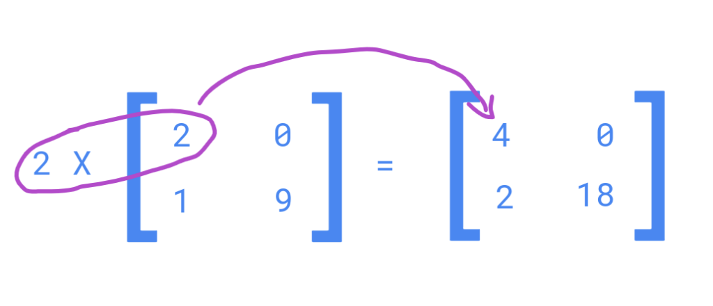
Multiplying a matrix by a single number (scalar) is straightforward. Simply multiply each element in the matrix by the multiplier.

For example, let’s multiply a matrix by 2:

When you multiply a matrix by another matrix, things get a bit trickier.

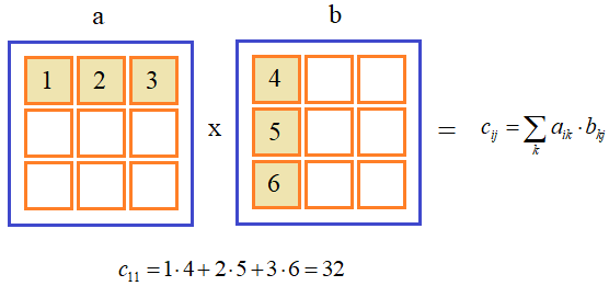
To multiply two matrices, take the dot product between each row on the left-hand side matrix and the column on the right-hand side matrix.

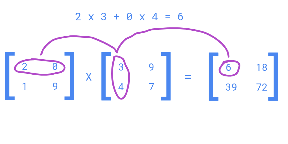
Here are all the calculations made to obtain the result matrix:

For a comprehensive explanation, feel free to check a more thorough guide on matrix multiplication here.

To keep it short, let’s move on to matrix multiplication in Python.

Matrix Multiplication in Python

To write a Python program that multiplies matrices, you need to implement a matrix multiplication algorithm.

Here is the pseudocode algorithm for matrix multiplication for matrices A and B of size N x M and M x P.

Let’s implement this logic in our Python program where a nested list represents a matrix.

In this example, we multiply a 3 x 3 matrix by a 3 x 4 matrix to get a 3 x 4 result matrix.

# 3 x 3 matrix A = [ [12,7,3], [4 ,5,6], [7 ,8,9] ] # 3 x 4 matrix B = [ [5,8,1,2], [6,7,3,0], [4,5,9,1] ] N = len(A) M = len(A[0]) P = len(B[0]) # Pre-fill the result matrix with 0s. # The size of the result is 3 x 4 (N x P). result = [] for i in range(N): row = [0] * P result.append(row) for i in range(N): for j in range(P): for k in range(M): result[i][j] += A[i][k] * B[k][j] for r in result: print(r)

[114, 160, 60, 27] [74, 97, 73, 14] [119, 157, 112, 23]

As you might already know, matrix multiplication is quite a common operation performed on matrices.

Thus, it would be a waste of time to implement this logic in each project where you need matrix multiplication.

This is where the @ operator comes to the rescue.

The @ Operator in Python

As of Python 3.5, it has been possible to specify a matrix multiplication operator @ to a custom class.

This happens by overriding the special method called __matmul__.

The idea is that when you call @ for two custom objects, the __matmul__ method gets triggered to calculate the result of matrix multiplication.

For instance, let’s create a custom class Matrix, and override the matrix multiplication method to it:

class Matrix(list): # Matrix multiplication A @ B def __matmul__(self, B): self = A N = len(A) M = len(A[0]) P = len(B[0]) result = [] for i in range(N): row = [0] * P result.append(row) for i in range(N): for j in range(P): for k in range(M): result[i][j] += A[i][k] * B[k][j] return result # Example A = Matrix([[2, 0],[1, 9]]) B = Matrix([[3, 9],[4, 7]]) print(A @ B)

As you can see, now it is possible to call @ between two matrix objects to multiply them.

And by the way, you could also directly call the __matmul__ method instead of using the @ shorthand.

# Example A = Matrix([[2, 0],[1, 9]]) B = Matrix([[3, 9],[4, 7]]) print(A.__matmul__(B))

Awesome. Now you understand how matrix multiplication works, and how to override the @ operator in your custom class.

Finally, let’s take a look at multiplying matrices with NumPy using the @ operator.

Matrix Multiplication with NumPy: A @ B

In data science, NumPy arrays are commonly used to represent matrices.

Because matrix multiplication is such a common operation to do, a NumPy array supports it by default.

This happens via the @ operator.

In other words, somewhere in the implementation of the NumPy array, there is a method called __matmul__ that implements matrix multiplication.

For example, let’s matrix-multiply two NumPy arrays:

import numpy as np A = np.array([[1, 2], [3, 4]]) B = np.array([[5, 6], [7, 8]]) product = A @ B print(product)

This concludes our example in matrix multiplication and @ operator in Python and NumPy.

Conclusion

Today you learned what is the @ operator in NumPy and Python.

To recap, as of Python 3.5, it has been possible to multiply matrices using the @ operator.

For instance, a NumPy array supports matrix multiplication with the @ operator.

To override/implement the behavior of the @ operator for a custom class, implement the __matmul__ method to the class. The __matmul__ method is called under the hood when calling @ between two objects.

Thanks for reading. Happy coding!

Источник