Opencv python gamma correction

I tried «gamma correction» of the image with Python + OpenCV

Image processing does not always provide beautiful images. It may contain dark objects or, conversely, images that are too bright. There is a method called gamma correction as a method of adjusting the brightness of an image.

This time, we will use Python to perform gamma correction of the image by OpenCV.

What is gamma correction?

** Gamma correction (or gamma conversion) ** is simply ** a method of adjusting the brightness of an image **.

The image generally contains dark and bright areas. In such a case, the feature of gamma correction is not to adjust the brightness at the same ratio for the entire image, but to adjust the brightness according to each pixel value. The gamma correction formula is as follows.

x is the input pixel value and y is the output pixel value. It is called gamma correction because the output changes depending on the value of $ \ gamma $ (gamma). If $ \ gamma $ is greater than 1, it will be brighter, and if it is less than 1, it will be darker.

The graph of gamma correction is as follows.

Preparation

The environment uses Google Colaboratory. The Python version is below.

import platform print("python " + platform.python_version()) # python 3.6.9 

Let’s display the image

In addition, import the following to display the image in Colaboratory.

from google.colab.patches import cv2_imshow 

Prepare a sample image as well. This time, we will use the free image from Pixabay.

Now, let’s display the prepared sample image.

img = cv2.imread(path) #path specifies where the image is placed cv2_imshow(img) 

Now let’s brighten the image using gamma correction. Create a gamma correction function in advance.

import numpy as np def create_gamma_img(gamma, img): gamma_cvt = np.zeros((256,1), dtype=np.uint8) for i in range(256): gamma_cvt[i][0] = 255*(float(i)/255)**(1.0/gamma) return cv2.LUT(img, gamma_cvt) 

Let’s display the gamma-corrected image side by side with the original image.

img_gamma = create_gamma_img(2, img) imgs = cv2.hconcat([img, img_gamma]) cv2_imshow(imgs) 

Make $ \ gamma $ greater than 1 to make it brighter. I tried it as 2 above.

Now, let’s change the value of $ \ gamma $ and display the gamma-corrected image.

img1 = create_gamma_img(0.33, img) img2 = create_gamma_img(0.5, img) img3 = create_gamma_img(0.66, img) img4 = create_gamma_img(1.5, img) img5 = create_gamma_img(2, img) img6 = create_gamma_img(3, img) imgs_1 = cv2.hconcat([img1, img2, img3]) imgs_2 = cv2.hconcat([img4, img5, img6]) imgs = cv2.vconcat([imgs_1, imgs_2]) cv2_imshow(imgs) 

From the upper left, the value of $ \ gamma $ was increased. The upper row is darker than the original image, and the lower row is brighter than the original image.

Summary

This time, I used Python to perform gamma correction (gamma conversion) on the image using OpenCV.

If you need to adjust the brightness of the image, try gamma correction.

For more details on gamma correction (gamma conversion), refer to the following.

Источник

Opencv python gamma correction

In this tutorial you will learn how to:

• Access pixel values
• Initialize a matrix with zeros
• Learn what cv::saturate_cast does and why it is useful
• Get some cool info about pixel transformations
• Improve the brightness of an image on a practical example

Theory

Note The explanation below belongs to the book Computer Vision: Algorithms and Applications by Richard Szeliski

Image Processing

• A general image processing operator is a function that takes one or more input images and produces an output image.
• Image transforms can be seen as:
  • Point operators (pixel transforms)
  • Neighborhood (area-based) operators

  Pixel Transforms

  • In this kind of image processing transform, each output pixel’s value depends on only the corresponding input pixel value (plus, potentially, some globally collected information or parameters).
  • Examples of such operators include brightness and contrast adjustments as well as color correction and transformations.

  Brightness and contrast adjustments

  • Two commonly used point processes are multiplication and addition with a constant: \[g(x) = \alpha f(x) + \beta\]
  • The parameters \(\alpha > 0\) and \(\beta\) are often called the gain and bias parameters; sometimes these parameters are said to control contrast and brightness respectively.
  • You can think of \(f(x)\) as the source image pixels and \(g(x)\) as the output image pixels. Then, more conveniently we can write the expression as: \[g(i,j) = \alpha \cdot f(i,j) + \beta\] where \(i\) and \(j\) indicates that the pixel is located in the i-th row and j-th column.

  Code

  • Downloadable code: Click here
  • The following code performs the operation \(g(i,j) = \alpha \cdot f(i,j) + \beta\) :

  // we’re NOT «using namespace std;» here, to avoid collisions between the beta variable and std::beta in c++17

  • Downloadable code: Click here
  • The following code performs the operation \(g(i,j) = \alpha \cdot f(i,j) + \beta\) :
  • Downloadable code: Click here
  • The following code performs the operation \(g(i,j) = \alpha \cdot f(i,j) + \beta\) :

  parser = argparse.ArgumentParser(description= ‘Code for Changing the contrast and brightness of an image! tutorial.’ )

  Explanation

  parser = argparse.ArgumentParser(description= ‘Code for Changing the contrast and brightness of an image! tutorial.’ )

  • Now, since we will make some transformations to this image, we need a new Mat object to store it. Also, we want this to have the following features:
    • Initial pixel values equal to zero
    • Same size and type as the original image

    We observe that cv::Mat::zeros returns a Matlab-style zero initializer based on image.size() and image.type()

    • Now, to perform the operation \(g(i,j) = \alpha \cdot f(i,j) + \beta\) we will access to each pixel in image. Since we are operating with BGR images, we will have three values per pixel (B, G and R), so we will also access them separately. Here is the piece of code:

    Notice the following (C++ code only):

    • To access each pixel in the images we are using this syntax: image.at(y,x)[c] where y is the row, x is the column and c is B, G or R (0, 1 or 2).
    • Since the operation \(\alpha \cdot p(i,j) + \beta\) can give values out of range or not integers (if \(\alpha\) is float), we use cv::saturate_cast to make sure the values are valid.
    • Finally, we create windows and show the images, the usual way.

    Note Instead of using the for loops to access each pixel, we could have simply used this command:

    where cv::Mat::convertTo would effectively perform *new_image = a*image + beta*. However, we wanted to show you how to access each pixel. In any case, both methods give the same result but convertTo is more optimized and works a lot faster.

    Result

    

    Practical example

    In this paragraph, we will put into practice what we have learned to correct an underexposed image by adjusting the brightness and the contrast of the image. We will also see another technique to correct the brightness of an image called gamma correction.

    Brightness and contrast adjustments

    Increasing (/ decreasing) the \(\beta\) value will add (/ subtract) a constant value to every pixel. Pixel values outside of the [0 ; 255] range will be saturated (i.e. a pixel value higher (/ lesser) than 255 (/ 0) will be clamped to 255 (/ 0)).

    

    The histogram represents for each color level the number of pixels with that color level. A dark image will have many pixels with low color value and thus the histogram will present a peak in its left part. When adding a constant bias, the histogram is shifted to the right as we have added a constant bias to all the pixels.

    

    Note that these histograms have been obtained using the Brightness-Contrast tool in the Gimp software. The brightness tool should be identical to the \(\beta\) bias parameters but the contrast tool seems to differ to the \(\alpha\) gain where the output range seems to be centered with Gimp (as you can notice in the previous histogram).

    It can occur that playing with the \(\beta\) bias will improve the brightness but in the same time the image will appear with a slight veil as the contrast will be reduced. The \(\alpha\) gain can be used to diminue this effect but due to the saturation, we will lose some details in the original bright regions.

    Gamma correction

    Gamma correction can be used to correct the brightness of an image by using a non linear transformation between the input values and the mapped output values:

    As this relation is non linear, the effect will not be the same for all the pixels and will depend to their original value.

    

    Correct an underexposed image

    The following image has been corrected with: \( \alpha = 1.3 \) and \( \beta = 40 \).

    

    The overall brightness has been improved but you can notice that the clouds are now greatly saturated due to the numerical saturation of the implementation used (highlight clipping in photography).

    The following image has been corrected with: \( \gamma = 0.4 \).

    

    The gamma correction should tend to add less saturation effect as the mapping is non linear and there is no numerical saturation possible as in the previous method.

    

    Left: histogram after alpha, beta correction ; Center: histogram of the original image ; Right: histogram after the gamma correction

    The previous figure compares the histograms for the three images (the y-ranges are not the same between the three histograms). You can notice that most of the pixel values are in the lower part of the histogram for the original image. After \( \alpha \), \( \beta \) correction, we can observe a big peak at 255 due to the saturation as well as a shift in the right. After gamma correction, the histogram is shifted to the right but the pixels in the dark regions are more shifted (see the gamma curves figure) than those in the bright regions.

    In this tutorial, you have seen two simple methods to adjust the contrast and the brightness of an image. They are basic techniques and are not intended to be used as a replacement of a raster graphics editor!

    Code

    Источник

    Discovering OpenCV with Python: Gamma correction

    Another practical exercise that I had quite some fun with was gamma correction. This concept is mainly used when we want to adjust the brightness of an image. We could also use it to restore the faded pictures to their previous depth of colour. Since I am just a Python Padawan, we will be demonstrating this on grayscale pictures but I promise, the concept works on coloured images as well. In this short article, I will focus on the restoration of faded pictures.

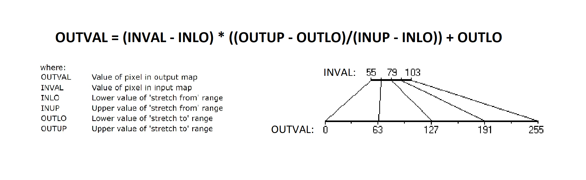
    A bit of (mathematical) background

    

    The logic behind is based on a concept called linear stretching. The faded picture simply means that the values of pixels are compressed to a smaller range and therefore not using the full range of values (in grayscale that would be from 0 to 255). For example, in the faded picture below, the values of the pixels range from 101 to 160. What linear stretching does, is that it re-scales the values to their full range from 0 to 255. Here is the mathematical formula on how this can be achieved with each value:

    Python implementation

    

    Just like in convolution, the necessary step is to cycle through every pixel and apply this mathematical formula to each of them. Be sure to check out my GitHub to see how it can be done. And voila, below is the result, look closely at how the histogram of pixel values stretched out from the original narrow range:

    Tool used to create histogram Hope you enjoyed the post, I recommend having a go at this and playing around with different images. Again, would appreciate if you let me know your thoughts. May the Python be with you.

    Источник

    Читайте также:  Javascript array to string separated by comma