Opencv convex hull python

Convex Hull using OpenCV in Python and C++

In this post, we will learn how to find the Convex Hull of a shape (a group of points). We will briefly explain the algorithm and then follow up with C++ and Python code implementation using OpenCV.

What is a Convex Hull?

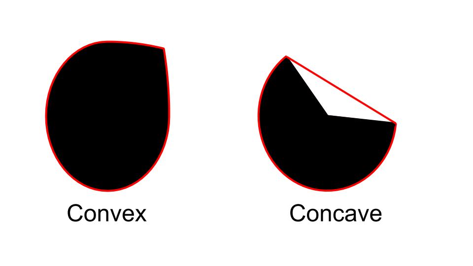
Let us break the term down into its two parts — Convex and Hull.

A Convex object is one with no interior angles greater than 180 degrees. A shape that is not convex is called Non-Convex or Concave. An example of a convex and a non-convex shape is shown in Figure 1.

Hull means the exterior or the shape of the object.

Therefore, the Convex Hull of a shape or a group of points is a tight fitting convex boundary around the points or the shape.

The Convex Hull of the two shapes in Figure 1 is shown in Figure 2. The Convex Hull of a convex object is simply its boundary. The Convex Hull of a concave shape is a convex boundary that most tightly encloses it.

Gift Wrapping Algorithms

Given a set of points that define a shape, how do we find its convex hull? The algorithms for finding the Convext Hull are often called Gift Wrapping algorithms. The video below explains a few algorithms with excellent animations:

Easy, huh? A lot of things look easy on the surface, but as soon as we impose certain constraints on them, things become pretty hard.

For example, the Jarvis March algorithm described in the video has complexity O(nh) where n is the number of input points and h is the number of points in the convex hull. Chan’s algorithm has complexity O(n log h).

Is an O(n) algorithm possible? The answer is YES, but boy the history of finding a linear algorithm for convex hull is a tad embrassing.

The first O(n) algorithm was published by Sklansky in 1972. It was later proven to be incorrect. Between 1972 and 1989, 16 different linear algorithms were published and 7 of them were found to be incorrect later on!

This reminds me of a joke I heard in college. Every difficult problem in mathematics has a simple, easy to understand wrong solution!

Now, here is an embarrassing icing on the embarrassing cake. The algorithm implemented in OpenCV is one by Sklansky (1982). It happens to be INCORRECT!

It is still a popular algorithm and in a vast majority of cases, it produces the right result. This algorithm is implemented in the convexHull class in OpenCV. Let’s now see how to use it.

convexHull in OpenCV

By now we know the Gift Wrapping algorithms for finding the Convex Hull work on a collection of points.

How do we use it on images?

We first need to binarize the image we are working with, find contours and finally find the convex hull. Let’s go step by step.

Download Code To easily follow along this tutorial, please download code by clicking on the button below. It’s FREE!

Step 1: Read the Input Image

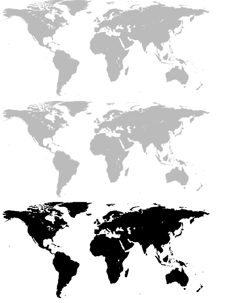
src = cv2.imread("sample.jpg", 1) # read input image

Mat src; src = imread("sample.jpg", 1); // read input image

Step 2: Binarize the input image

We perform binarization in three steps —

The results of these steps are shown in Figure 3. And here is the code.

gray = cv2.cvtColor(src, cv2.COLOR_BGR2GRAY) # convert to grayscale blur = cv2.blur(gray, (3, 3)) # blur the image ret, thresh = cv2.threshold(blur, 50, 255, cv2.THRESH_BINARY)

Mat gray, blur_image, threshold_output; cvtColor(src, gray, COLOR_BGR2GRAY); // convert to grayscale blur(gray, blur_image, Size(3, 3)); // apply blur to grayscaled image threshold(blur_image, threshold_output, 50, 255, THRESH_BINARY); // apply binary thresholding

As you can see, we have converted the image into binary blobs. We next need to find the boundaries of these blobs.

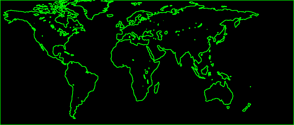
Step 3: Use findContour to find contours

Next, we find the contour around every continent using the findContour function in OpenCV. Finding the contours gives us a list of boundary points around each blob.

If you are a beginner, you may be tempted to think why we did not simply use edge detection? Edge detection would have simply given us locations of the edges. But we are interested in finding how edges are connected to each other. findContour allows us to find those connections and returns the points that form a contour as a list.

# Finding contours for the thresholded image im2, contours, hierarchy = cv2.findContours(thresh, cv2.RETR_TREE, cv2.CHAIN_APPROX_SIMPLE)

vector < vector> contours; // list of contour points vector hierarchy; // find contours findContours(threshold_output, contours, hierarchy, RETR_TREE, CHAIN_APPROX_SIMPLE, Point(0, 0));

Step 4: Find the Convex Hull using convexHull

Since we have found the contours, we can now find the Convex Hull for each of the contours. This can be done using convexHull function.

# create hull array for convex hull points hull = [] # calculate points for each contour for i in range(len(contours)): # creating convex hull object for each contour hull.append(cv2.convexHull(contours[i], False))

// create hull array for convex hull points vector < vector> hull(contours.size()); for(int i = 0; i < contours.size(); i++) convexHull(Mat(contours[i]), hull[i], False);

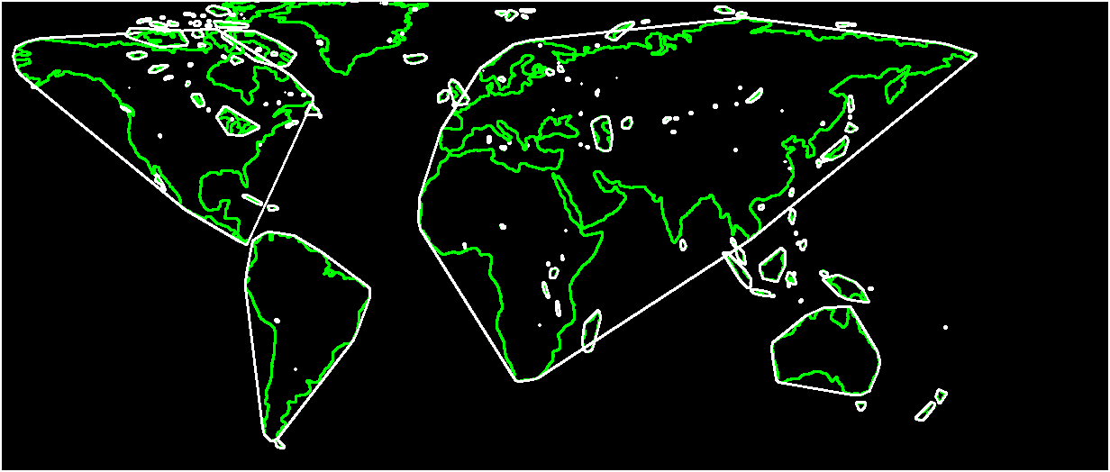
Step 5: Draw the Convex Hull

The final step is to visualize the convex hulls we have just found. Of course a convex hull itself is just a contour and therefore we can use OpenCV’s drawContours.

# create an empty black image drawing = np.zeros((thresh.shape[0], thresh.shape[1], 3), np.uint8) # draw contours and hull points for i in range(len(contours)): color_contours = (0, 255, 0) # green - color for contours color = (255, 0, 0) # blue - color for convex hull # draw ith contour cv2.drawContours(drawing, contours, i, color_contours, 1, 8, hierarchy) # draw ith convex hull object cv2.drawContours(drawing, hull, i, color, 1, 8)

// create a blank image (black image) Mat drawing = Mat::zeros(threshold_output.size(), CV_8UC3); for(int i = 0; i < contours.size(); i++) [ Scalar color_contours = Scalar(0, 255, 0); // green - color for contours Scalar color = Scalar(255, 0, 0); // blue - color for convex hull // draw ith contour drawContours(drawing, contours, i, color_contours, 1, 8, vector(), 0, Point()); // draw ith convex hull drawContours(drawing, hull, i, color, 1, 8, vector(), 0, Point()); >

Applications of Convex Hull

There are several applications of the convex hull. Let’s explore a couple of them.

Boundary from a set of points

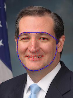
Regular readers of this blog may be aware we have used convexHull before in our face swap application. Given the facial landmarks detected using Dlib, we found the boundary of the face using the convex hull as shown in Figure 6.

There are several other applications, where we recover feature points information instead of contour information. For example, in many active lighting systems like Kinect, we recover a grayscale depth map that is a collection of points. We can use the convex hull of these points to locate the boundary of an object in the scene.

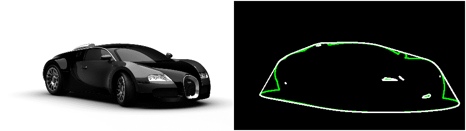
Collision Avoidance

Imagine a car as a set of points and the polygon (minimal set) containing all the points. Now if the convex hull is able to avoid the obstacles, so should the car. Finding the intersection between arbitrary contours is computationally much more expensive than finding the collision between two convex polygons. So you are better off using a convex hull for collision detection or avoidance.

Subscribe & Download Code

If you liked this article and would like to download code (C++ and Python) and example images used in this post, please click here. Alternately, sign up to receive a free Computer Vision Resource Guide. In our newsletter, we share OpenCV tutorials and examples written in C++/Python, and Computer Vision and Machine Learning algorithms and news.

References and Further Reading

Источник

Opencv convex hull python

In this article, we will learn

• To find the different features of contours, like area, perimeter, centroid, bounding box etc
• You will see plenty of functions related to contours.

1. Moments

Image moments help you to calculate some features like center of mass of the object, area of the object etc. Check out the wikipedia page on Image Moments

The function cv.moments() gives a dictionary of all moment values calculated. See below:

From this moments, you can extract useful data like area, centroid etc. Centroid is given by the relations, \(C_x = \frac>>\) and \(C_y = \frac>>\). This can be done as follows:

2. Contour Area

Contour area is given by the function cv.contourArea() or from moments, M['m00'].

3. Contour Perimeter

It is also called arc length. It can be found out using cv.arcLength() function. Second argument specify whether shape is a closed contour (if passed True), or just a curve.

4. Contour Approximation

It approximates a contour shape to another shape with less number of vertices depending upon the precision we specify. It is an implementation of Douglas-Peucker algorithm. Check the wikipedia page for algorithm and demonstration.

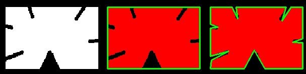
To understand this, suppose you are trying to find a square in an image, but due to some problems in the image, you didn't get a perfect square, but a "bad shape" (As shown in first image below). Now you can use this function to approximate the shape. In this, second argument is called epsilon, which is maximum distance from contour to approximated contour. It is an accuracy parameter. A wise selection of epsilon is needed to get the correct output.

Below, in second image, green line shows the approximated curve for epsilon = 10% of arc length. Third image shows the same for epsilon = 1% of the arc length. Third argument specifies whether curve is closed or not.

5. Convex Hull

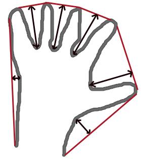
Convex Hull will look similar to contour approximation, but it is not (Both may provide same results in some cases). Here, cv.convexHull() function checks a curve for convexity defects and corrects it. Generally speaking, convex curves are the curves which are always bulged out, or at-least flat. And if it is bulged inside, it is called convexity defects. For example, check the below image of hand. Red line shows the convex hull of hand. The double-sided arrow marks shows the convexity defects, which are the local maximum deviations of hull from contours.

There is a little bit things to discuss about it its syntax:

• points are the contours we pass into.
• hull is the output, normally we avoid it.
• clockwise : Orientation flag. If it is True, the output convex hull is oriented clockwise. Otherwise, it is oriented counter-clockwise.
• returnPoints : By default, True. Then it returns the coordinates of the hull points. If False, it returns the indices of contour points corresponding to the hull points.

So to get a convex hull as in above image, following is sufficient:

But if you want to find convexity defects, you need to pass returnPoints = False. To understand it, we will take the rectangle image above. First I found its contour as cnt. Now I found its convex hull with returnPoints = True, I got following values: [[[234 202]], [[ 51 202]], [[ 51 79]], [[234 79]]] which are the four corner points of rectangle. Now if do the same with returnPoints = False, I get following result: [[129],[ 67],[ 0],[142]]. These are the indices of corresponding points in contours. For eg, check the first value: cnt[129] = [[234, 202]] which is same as first result (and so on for others).

You will see it again when we discuss about convexity defects.

6. Checking Convexity

There is a function to check if a curve is convex or not, cv.isContourConvex(). It just return whether True or False. Not a big deal.

7. Bounding Rectangle

There are two types of bounding rectangles.

7.a. Straight Bounding Rectangle

It is a straight rectangle, it doesn't consider the rotation of the object. So area of the bounding rectangle won't be minimum. It is found by the function cv.boundingRect().

Let (x,y) be the top-left coordinate of the rectangle and (w,h) be its width and height.

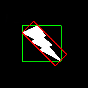
7.b. Rotated Rectangle

Here, bounding rectangle is drawn with minimum area, so it considers the rotation also. The function used is cv.minAreaRect(). It returns a Box2D structure which contains following details - ( center (x,y), (width, height), angle of rotation ). But to draw this rectangle, we need 4 corners of the rectangle. It is obtained by the function cv.boxPoints()

Both the rectangles are shown in a single image. Green rectangle shows the normal bounding rect. Red rectangle is the rotated rect.

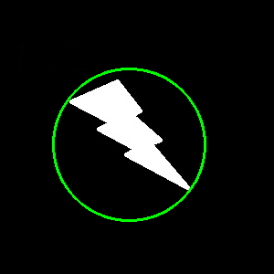
8. Minimum Enclosing Circle

Next we find the circumcircle of an object using the function cv.minEnclosingCircle(). It is a circle which completely covers the object with minimum area.

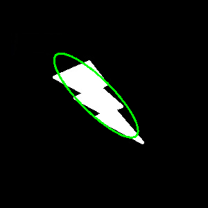
9. Fitting an Ellipse

Next one is to fit an ellipse to an object. It returns the rotated rectangle in which the ellipse is inscribed.

10. Fitting a Line

Similarly we can fit a line to a set of points. Below image contains a set of white points. We can approximate a straight line to it.

Источник