Метод условного градиента python

Градиентный спуск в Python

Рабочая область функции (заданный интервал) разбита на несколько точек. Выбраны точки локальных минимумов. После этого все координаты передаются функции в качестве аргументов и выбирается аргумент, дающий наименьшее значение. Затем применяется метод градиентного спуска.

Реализация

Прежде всего, numpy необходим для функций sinus, cosinus и exp. Также необходимо добавить matplotlib для построения графиков.

import numpy as np import matplotlib.pyplot as plot

radius = 8 # working plane radius centre = (global_epsilon, global_epsilon) # centre of the working circle arr_shape = 100 # number of points processed / 360 step = radius / arr_shape # step between two points

arr_shape должна быть 100, потому что, если она больше, программа начинает работать значительно медленнее. И не может быть меньше, иначе это испортит расчеты.

Функция, для которой рассчитывается минимум:

def differentiable_function(x, y): return np.sin(x) * np.exp((1 - np.cos(y)) ** 2) + \ np.cos(y) * np.exp((1 - np.sin(x)) ** 2) + (x - y) ** 2

Затем выбирается приращение аргумента:

Поскольку предел аргумента стремится к нулю, точность должна быть небольшой по сравнению с радиусом рабочей плоскости:

global_epsilon = 0.000000001 # argument increment for derivative

Для дальнейшего разбиения плоскости необходим поворот вектора:

Если вращение применяется к вектору (x, 0), повернутый вектор будет вычисляться следующим образом:

def rotate_vector(length, a): return length * np.cos(a), length * np.sin(a)

Расчет производной по оси Y, где эпсилон — значение y:

def derivative_y(epsilon, arg): return (differentiable_function(arg, epsilon + global_epsilon) - differentiable_function(arg, epsilon)) / global_epsilon

Вычисление производной по оси X, где эпсилон — значение x:

def derivative_x(epsilon, arg): return (differentiable_function(global_epsilon + epsilon, arg) - differentiable_function(epsilon, arg)) / global_epsilon

Поскольку градиент вычисляется для 2D-функции, k равно нулю

gradient = derivative_x(x, y) + derivative_y(y, x)

Возвращаемое значение представляет собой массив приблизительных локальных минимумов.

Локальный минимум распознается по смене знака производной с минуса на плюс. Подробнее об этом здесь: https://en.wikipedia.org/wiki/Maxima_and_minima

def calculate_flip_points(): flip_points = np.array([0, 0]) points = np.zeros((360, arr_shape), dtype=bool) cx, cy = centre for i in range(arr_shape): for alpha in range(360): x, y = rotate_vector(step, alpha) x = x * i + cx y = y * i + cy points[alpha][i] = derivative_x(x, y) + derivative_y(y, x) > 0 if not points[alpha][i - 1] and points[alpha][i]: flip_points = np.vstack((flip_points, np.array([alpha, i - 1]))) return flip_points

Выбор точки из flip_points, значение функции от которой минимально:

def pick_estimates(positions): vx, vy = rotate_vector(step, positions[1][0]) cx, cy = centre best_x, best_y = cx + vx * positions[1][1], cy + vy * positions[1][1] for index in range(2, len(positions)): vx, vy = rotate_vector(step, positions[index][0]) x, y = cx + vx * positions[index][1], cy + vy * positions[index][1] if differentiable_function(best_x, best_y) > differentiable_function(x, y): best_x = x best_y = y for index in range(360): vx, vy = rotate_vector(step, index) x, y = cx + vx * (arr_shape - 1), cy + vy * (arr_shape - 1) if differentiable_function(best_x, best_y) > differentiable_function(x, y): best_x = x best_y = y return best_x, best_y

Метод градиентного спуска:

def gradient_descent(best_estimates, is_x): derivative = derivative_x if is_x else derivative_y best_x, best_y = best_estimates descent_step = step value = derivative(best_y, best_x) while abs(value) > global_epsilon: descent_step *= 0.95 best_y = best_y - descent_step \ if derivative(best_y, best_x) > 0 else best_y + descent_step value = derivative(best_y, best_x) return best_y, best_x

Нахождение точки минимума:

def find_minimum(): return gradient_descent(gradient_descent(pick_estimates(calculate_flip_points()), False), True)

Формирование сетки точек для построения:

def get_grid(grid_step): samples = np.arange(-radius, radius, grid_step) x, y = np.meshgrid(samples, samples) return x, y, differentiable_function(x, y)

def draw_chart(point, grid): point_x, point_y, point_z = point grid_x, grid_y, grid_z = grid plot.rcParams.update(< 'figure.figsize': (4, 4), 'figure.dpi': 200, 'xtick.labelsize': 4, 'ytick.labelsize': 4 >) ax = plot.figure().add_subplot(111, projection='3d') ax.scatter(point_x, point_y, point_z, color='red') ax.plot_surface(grid_x, grid_y, grid_z, rstride=5, cstride=5, alpha=0.7) plot.show()

if __name__ == '__main__': min_x, min_y = find_minimum() minimum = (min_x, min_y, differentiable_function(min_x, min_y)) draw_chart(minimum, get_grid(0.05))

Заключение

Процесс вычисления минимального значения с помощью алгоритма может быть не очень точным при вычислениях в более крупном масштабе, например, если радиус рабочей плоскости равен 1000, но он очень быстрый по сравнению с точным. Плюс в любом случае, если радиус большой, результат находится примерно в том положении, в котором он должен быть, поэтому разница не будет заметна на графике.

Исходный код:

import numpy as np import matplotlib.pyplot as plot radius = 8 # working plane radius global_epsilon = 0.000000001 # argument increment for derivative centre = (global_epsilon, global_epsilon) # centre of the working circle arr_shape = 100 # number of points processed / 360 step = radius / arr_shape # step between two points def differentiable_function(x, y): return np.sin(x) * np.exp((1 - np.cos(y)) ** 2) + \ np.cos(y) * np.exp((1 - np.sin(x)) ** 2) + (x - y) ** 2 def rotate_vector(length, a): return length * np.cos(a), length * np.sin(a) def derivative_x(epsilon, arg): return (differentiable_function(global_epsilon + epsilon, arg) - differentiable_function(epsilon, arg)) / global_epsilon def derivative_y(epsilon, arg): return (differentiable_function(arg, epsilon + global_epsilon) - differentiable_function(arg, epsilon)) / global_epsilon def calculate_flip_points(): flip_points = np.array([0, 0]) points = np.zeros((360, arr_shape), dtype=bool) cx, cy = centre for i in range(arr_shape): for alpha in range(360): x, y = rotate_vector(step, alpha) x = x * i + cx y = y * i + cy points[alpha][i] = derivative_x(x, y) + derivative_y(y, x) > 0 if not points[alpha][i - 1] and points[alpha][i]: flip_points = np.vstack((flip_points, np.array([alpha, i - 1]))) return flip_points def pick_estimates(positions): vx, vy = rotate_vector(step, positions[1][0]) cx, cy = centre best_x, best_y = cx + vx * positions[1][1], cy + vy * positions[1][1] for index in range(2, len(positions)): vx, vy = rotate_vector(step, positions[index][0]) x, y = cx + vx * positions[index][1], cy + vy * positions[index][1] if differentiable_function(best_x, best_y) > differentiable_function(x, y): best_x = x best_y = y for index in range(360): vx, vy = rotate_vector(step, index) x, y = cx + vx * (arr_shape - 1), cy + vy * (arr_shape - 1) if differentiable_function(best_x, best_y) > differentiable_function(x, y): best_x = x best_y = y return best_x, best_y def gradient_descent(best_estimates, is_x): derivative = derivative_x if is_x else derivative_y best_x, best_y = best_estimates descent_step = step value = derivative(best_y, best_x) while abs(value) > global_epsilon: descent_step *= 0.95 best_y = best_y - descent_step \ if derivative(best_y, best_x) > 0 else best_y + descent_step value = derivative(best_y, best_x) return best_y, best_x def find_minimum(): return gradient_descent(gradient_descent(pick_estimates(calculate_flip_points()), False), True) def get_grid(grid_step): samples = np.arange(-radius, radius, grid_step) x, y = np.meshgrid(samples, samples) return x, y, differentiable_function(x, y) def draw_chart(point, grid): point_x, point_y, point_z = point grid_x, grid_y, grid_z = grid plot.rcParams.update(< 'figure.figsize': (4, 4), 'figure.dpi': 200, 'xtick.labelsize': 4, 'ytick.labelsize': 4 >) ax = plot.figure().add_subplot(111, projection='3d') ax.scatter(point_x, point_y, point_z, color='red') ax.plot_surface(grid_x, grid_y, grid_z, rstride=5, cstride=5, alpha=0.7) plot.show() if __name__ == '__main__': min_x, min_y = find_minimum() minimum = (min_x, min_y, differentiable_function(min_x, min_y)) draw_chart(minimum, get_grid(0.05))

Источник

Решение задачи Марковица, при ограничении на короткую продажу методом условного градиента

Решение задачи Марковица, при ограничении на короткую продажу методом условного градиента
Помогите решить задачу Марковица, при ограничении на короткую продажу методом условного градиента.

Решение задачи оптимального управления в параболических уравнениях методом условного градиента
Здравствуйте, увааемые форумчане! Для сдачи диплома необходимо мне написать прогу, которая решает.

Методы: условного градиента, проекции градиента, возможных направлений
Помогите плиз с кодом. метод условного градиента метод проекции градиента метод возможных.

Решение систем нелинейных уравнений Методом градиента (ошибка в коде)
Доброго времени суток! Решил набрать простой код для метода быстрого спуска( подъёма ) по.

Метод условного градиента
Здравствуйте, уважаемые жители сyberforum.Передо мной стоит следующая задача реализовать метод.

Метод условного градиента
Для решения методом условного градиента с начальными приближением _ найти решение первой.

Реализация метода условного градиента
Всем привет! помогите пожалуйста решить задачку кто может. Задача Реализуйте метод условного.

Исправить ошибку, которая в программе для метода условного градиента
Добрый день! Помогите исправить ошибку, которая в программе для метода условного градиента

Методом градиента исследовать на экстремум указанную функцию при указанных ограничениях.
Помогите, пожалуйста. Гугл ничего внятного не дал понять. Методом градиента исследовать на.

Решение задачи симплекс методом
Всем доброго времени суток. Помогите, пожалуйста, при компиляции выдает такую ошибку:" fatal error.

Источник

Linear Regression using Stochastic Gradient Descent in Python

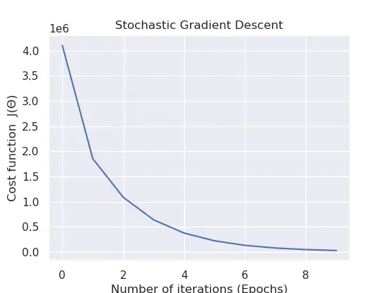
In today’s tutorial, we will learn about the basic concept of another iterative optimization algorithm called the stochastic gradient descent and how to implement the process from scratch. You will also see some benefits and drawbacks behind the algorithm.

If you aren’t aware of the gradient descent algorithm, please see the most recent tutorial before you continue reading.

The Concept behind Stochastic Descent Descent

One of the significant downsides behind the gradient descent algorithm is when you are working with a lot of samples. You might be wondering why this poses a problem.

The reason behind this is because we need to compute first the sum of squared residuals on as many samples, multiplied by the number of features. Then compute the derivative of this function for each of the features within our dataset. This will undoubtedly require a lot of computation power if your training set is significantly large and when you want better results.

Considering that gradient descent is a repetitive algorithm, this needs to be processed for as many iterations as specified. That’s dreadful , isn’t it? Instead of relying on gradient descent for each example, an easy solution is to have a different approach. This approach would be computing the loss/cost over a small random sample of the training data, calculating the derivative of that sample, and assuming that the derivative is the best direction to make gradient descent.

Along with this, as opposed to selecting a random data point, we pick a random ordering over the information and afterward walk conclusively through them. This advantageous variant of gradient descent is called stochastic gradient descent.

In some cases, it may not go in the optimal direction, which could affect the loss/cost negatively. Nevertheless, this can be taken care of by running the algorithm repetitively and by taking little actions as we iterate.

Applying Stochastic Gradient Descent with Python

Now that we understand the essentials concept behind stochastic gradient descent let’s implement this in Python on a randomized data sample.

Open a brand-new file, name it linear_regression_sgd.py, and insert the following code:

Источник