Метод ньютона оптимизация python

Newton’s method with 10 lines of Python

Newton’s method, which is an old numerical approximation technique that could be used to find the roots of complex polynomials and any differentiable function. We’ll code it up in 10 lines of Python in this post.

Let’s say we have a complicated polynomial:

and we want to find its roots. Unfortunately we know from the Galois theory that there is no formula for a 5th degree polynomial so we’ll have to use numeric methods. Wait a second. What’s going on? We all learned the quadratic formula in school, and there are formulas for cubic and quartic polynomials, but Galois proved that no such «root-finding» formula exist for fifth or higher degree polynomials, that uses only the usual algebraic operations (addition, subtraction, multiplication, division) and application of radicals (square roots, cube roots, etc).

Bit more maths context

Some nice guys pointed out on reddit that I didn’t quite get the theory right. Sorry about that, I’m no mathematician by any means. It turns out that this polynomial could be factored into $latex x^2(x-1)(6x^2 + x — 3)$ and solved with traditional cubic formula.

Also the theorem I referred to is the Abel-Ruffini Theorem and it only applies to the solution to the general polynomial of degree five or greater. Nonetheless the example is still valid, and demonstrates how would you apply Newton’s method, to any polynomial, so let’s crack on.

Simplest way to solve it

So in these cases we have to resort to numeric linear approximation. A simple way would be to use the intermediate value theorem, which states that if $latex f(x)$ is continuous on $latex [a,b]$ and $latex f(a) < y< f(b)$, then there is an $latex x$ between $latex a$ and $latex b$ so that $latex f(x)=y$.

We could exploit this by looking for an $latex x_1$ where $latex f(x_1)>0$ and an $latex x_2$ where $latex f(x_2)$, and find that $latex f(x_3)$ will be positive, then continue with$latex x_4=\frac$ which would be negative and our proposed $latex x_n$ would become closer and closer to $latex f(x_n)=0$. This method however can be pretty slow, so Newton devised a better way to speed things up (when it works).

How Newton solved it

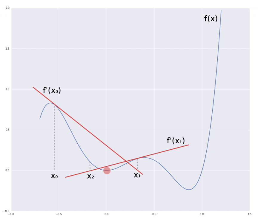
If you look at the figure below, you’ll see the plot of our polynomial. It has three roots at 0, 1, and somewhere in-between. So how do we find these?

In Newton’s method we take a random point $latex f(x_0)$, then draw a tangent line through $latex x_0, f(x_0)$, using the derivative $latex f'(x_0)$. The point $latex x_1$ where this tangent line crosses the $latex x$ axis will become the next proposal we check. We calculate the tangent line at $latex f'(x_1)$ and find $latex x_2$. We carry on, and as we do $latex |f(x_n)| \to 0$, or in other words we can make our approximation as close to zero as we want, provided we are willing to continue with the number crunching. Using the fact that the slope of tangent (by the definition of derivatives) at $latex x_n$ is $latex f'(x_n)$ we can derive the formula for $latex x_$, i.e. where the tangent crosses the $latex x$ axis:

Code

With all this in mind it’s easy to write an algorithm that approximates $f(x)=0$ with arbitrary error $latex \varepsilon$. Obviously in this example depending on where we start $latex x_0$ we might find different roots.

def dx(f, x): return abs(0-f(x)) def newtons_method(f, df, x0, e): delta = dx(f, x0) while delta > e: x0 = x0 - f(x0)/df(x0) delta = dx(f, x0) print 'Root is at: ', x0 print 'f(x) at root is: ', f(x0) 

There you go, we’are done in 10 lines (9 without the blank line), even less without the print statements.

In use

So in order to use this, we need two functions, $latex f(x)$ and $latex f'(x)$. For this polynomial these are:

def f(x): return 6*x**5-5*x**4-4*x**3+3*x**2 def df(x): return 30*x**4-20*x**3-12*x**2+6*x 

Now we can simply find the three roots with:

x0s = [0, .5, 1] for x0 in x0s: newtons_method(f, df, x0, 1e-5) # Root is at: 0 # f(x) at root is: 0 # Root is at: 0.628668078167 # f(x) at root is: -1.37853879978e-06 # Root is at: 1 # f(x) at root is: 0 

Summary

All of the above code, and some additional comparison test with the scipy.optimize.newton method can be found in this Gist. And don’t forget, if you find it too much trouble differentiating your functions, just use SymPy, I wrote about it here.

Newton’s method is pretty powerful but there could be problems with the speed of convergence, and awfully wrong initial guesses might make it not even converge ever, see here. Nonetheless I hope you found this relatively useful.. Let me know in the comments.

Updated: February 9, 2016

Источник

scipy.optimize.newton#

Find a root of a real or complex function using the Newton-Raphson (or secant or Halley’s) method.

Find a root of the scalar-valued function func given a nearby scalar starting point x0. The Newton-Raphson method is used if the derivative fprime of func is provided, otherwise the secant method is used. If the second order derivative fprime2 of func is also provided, then Halley’s method is used.

If x0 is a sequence with more than one item, newton returns an array: the roots of the function from each (scalar) starting point in x0. In this case, func must be vectorized to return a sequence or array of the same shape as its first argument. If fprime (fprime2) is given, then its return must also have the same shape: each element is the first (second) derivative of func with respect to its only variable evaluated at each element of its first argument.

newton is for finding roots of a scalar-valued functions of a single variable. For problems involving several variables, see root .

Parameters : func callable

The function whose root is wanted. It must be a function of a single variable of the form f(x,a,b,c. ) , where a,b,c. are extra arguments that can be passed in the args parameter.

x0 float, sequence, or ndarray

An initial estimate of the root that should be somewhere near the actual root. If not scalar, then func must be vectorized and return a sequence or array of the same shape as its first argument.

fprime callable, optional

The derivative of the function when available and convenient. If it is None (default), then the secant method is used.

args tuple, optional

Extra arguments to be used in the function call.

tol float, optional

The allowable error of the root’s value. If func is complex-valued, a larger tol is recommended as both the real and imaginary parts of x contribute to |x — x0| .

maxiter int, optional

Maximum number of iterations.

fprime2 callable, optional

The second order derivative of the function when available and convenient. If it is None (default), then the normal Newton-Raphson or the secant method is used. If it is not None, then Halley’s method is used.

x1 float, optional

Another estimate of the root that should be somewhere near the actual root. Used if fprime is not provided.

rtol float, optional

Tolerance (relative) for termination.

full_output bool, optional

If full_output is False (default), the root is returned. If True and x0 is scalar, the return value is (x, r) , where x is the root and r is a RootResults object. If True and x0 is non-scalar, the return value is (x, converged, zero_der) (see Returns section for details).

disp bool, optional

If True, raise a RuntimeError if the algorithm didn’t converge, with the error message containing the number of iterations and current function value. Otherwise, the convergence status is recorded in a RootResults return object. Ignored if x0 is not scalar. Note: this has little to do with displaying, however, the `disp` keyword cannot be renamed for backwards compatibility.

Returns : root float, sequence, or ndarray

Estimated location where function is zero.

r RootResults , optional

Present if full_output=True and x0 is scalar. Object containing information about the convergence. In particular, r.converged is True if the routine converged.

converged ndarray of bool, optional

Present if full_output=True and x0 is non-scalar. For vector functions, indicates which elements converged successfully.

zero_der ndarray of bool, optional

Present if full_output=True and x0 is non-scalar. For vector functions, indicates which elements had a zero derivative.

interface to root solvers for scalar functions

interface to root solvers for multi-input, multi-output functions

The convergence rate of the Newton-Raphson method is quadratic, the Halley method is cubic, and the secant method is sub-quadratic. This means that if the function is well-behaved the actual error in the estimated root after the nth iteration is approximately the square (cube for Halley) of the error after the (n-1)th step. However, the stopping criterion used here is the step size and there is no guarantee that a root has been found. Consequently, the result should be verified. Safer algorithms are brentq, brenth, ridder, and bisect, but they all require that the root first be bracketed in an interval where the function changes sign. The brentq algorithm is recommended for general use in one dimensional problems when such an interval has been found.

When newton is used with arrays, it is best suited for the following types of problems:

• The initial guesses, x0, are all relatively the same distance from the roots.
• Some or all of the extra arguments, args, are also arrays so that a class of similar problems can be solved together.
• The size of the initial guesses, x0, is larger than O(100) elements. Otherwise, a naive loop may perform as well or better than a vector.

>>> import numpy as np >>> import matplotlib.pyplot as plt >>> from scipy import optimize 

>>> def f(x): . return (x**3 - 1) # only one real root at x = 1 

fprime is not provided, use the secant method:

>>> root = optimize.newton(f, 1.5) >>> root 1.0000000000000016 >>> root = optimize.newton(f, 1.5, fprime2=lambda x: 6 * x) >>> root 1.0000000000000016 

Only fprime is provided, use the Newton-Raphson method:

>>> root = optimize.newton(f, 1.5, fprime=lambda x: 3 * x**2) >>> root 1.0 

Both fprime2 and fprime are provided, use Halley’s method:

>>> root = optimize.newton(f, 1.5, fprime=lambda x: 3 * x**2, . fprime2=lambda x: 6 * x) >>> root 1.0 

When we want to find roots for a set of related starting values and/or function parameters, we can provide both of those as an array of inputs:

>>> f = lambda x, a: x**3 - a >>> fder = lambda x, a: 3 * x**2 >>> rng = np.random.default_rng() >>> x = rng.standard_normal(100) >>> a = np.arange(-50, 50) >>> vec_res = optimize.newton(f, x, fprime=fder, args=(a, ), maxiter=200) 

The above is the equivalent of solving for each value in (x, a) separately in a for-loop, just faster:

>>> loop_res = [optimize.newton(f, x0, fprime=fder, args=(a0,), . maxiter=200) . for x0, a0 in zip(x, a)] >>> np.allclose(vec_res, loop_res) True 

Plot the results found for all values of a :

>>> analytical_result = np.sign(a) * np.abs(a)**(1/3) >>> fig, ax = plt.subplots() >>> ax.plot(a, analytical_result, 'o') >>> ax.plot(a, vec_res, '.') >>> ax.set_xlabel('$a$') >>> ax.set_ylabel('$x$ where $f(x, a)=0$') >>> plt.show() 

Источник

How to use the Newton’s method in python ?

In numerical analysis, Newton’s method (also known as the Newton–Raphson method), named after Isaac Newton and Joseph Raphson, is a method for finding successively better approximations to the roots (or zeroes) of a real-valued function. wikipedia. Example of implementation using python:

Solution 1

from scipy import misc def NewtonsMethod(f, x, tolerance=0.000001): while True: x1 = x - f(x) / misc.derivative(f, x) t = abs(x1 - x) if t < tolerance: break x = x1 return x def f(x): return (1.0/4.0)*x**3+(3.0/4.0)*x**2-(3.0/2.0)*x-2 x = 4 x0 = NewtonsMethod(f, x) print('x: ', x) print('x0: ', x0) print("f(x0) = ", ((1.0/4.0)*x0**3+(3.0/4.0)*x0**2-(3.0/2.0)*x0-2 )) 

x: 4 x0: 2.0000002745869883 f(x0) = 1.2356416165815176e-06 

Solution 2 (scipy)

from scipy.optimize import newton def f(x): return (1.0/4.0)*x**3+(3.0/4.0)*x**2-(3.0/2.0)*x-2 x = 4 x0 = newton(f, x, fprime=None, args=(), tol=1.48e-08, maxiter=50, fprime2=None) print('x: ', x) print('x0: ', x0) print("f(x0) = ", ((1.0/4.0)*x0**3+(3.0/4.0)*x0**2-(3.0/2.0)*x0-2 )) 

x: 4 x0: 2.000000000000008 f(x0) = 3.597122599785507e-14 

Plot the above figure using matplotlib

#!/usr/bin/env python from pylab import * t = arange(-6.0, 4.0, 0.01) s= t*t*t/4.0+3.0*t*t/4.0-3*t/2.0-2.0 ax = subplot(111) ax.plot(t, s) ax.scatter([-4,-1,2],[0,0,0]) ax.grid(True) ax.spines['left'].set_position('zero') ax.spines['right'].set_color('none') ax.spines['bottom'].set_position('zero') ax.spines['top'].set_color('none') ax.set_xlim(-6,6) ax.set_ylim(-20,20) text(-3.0, 12, r"$f(x)=(1/4)*X^3+(3/4)*X^2-(3/2)*X-2$", horizontalalignment='center', fontsize=8) plt.title("How to implement the Newton's method using python \n for finding the zeroes of a real-valued function",fontsize=10) plt.xticks(fontsize=8) plt.yticks(fontsize=8) plt.savefig('NewtonMethodExemple.png') show() 

Note: with numpy it is also possible to find the root of a polynomial with root, example the following polynomial has 3 roots:

>>> import numpy as np >>> coeff = [1.0/4.0,3.0/4.0,-3.0/2.0,-2] >>> np.roots(coeff) array([-4., 2., -1.]) 

References

Источник