Matplotlib python цвет фона

Specifying colors#

Matplotlib recognizes the following formats to specify a color.

RGB or RGBA (red, green, blue, alpha) tuple of float values in a closed interval [0, 1].

Case-insensitive hex RGB or RGBA string.

Case-insensitive RGB or RGBA string equivalent hex shorthand of duplicated characters.

String representation of float value in closed interval [0, 1] for grayscale values.

Single character shorthand notation for some basic colors.

The colors green, cyan, magenta, and yellow do not coincide with X11/CSS4 colors. Their particular shades were chosen for better visibility of colored lines against typical backgrounds.

• ‘b’ as blue
• ‘g’ as green
• ‘r’ as red
• ‘c’ as cyan
• ‘m’ as magenta
• ‘y’ as yellow
• ‘k’ as black
• ‘w’ as white

Case-insensitive X11/CSS4 color name with no spaces.

Case-insensitive color name from xkcd color survey with ‘xkcd:’ prefix.

Case-insensitive Tableau Colors from ‘T10’ categorical palette.

This is the default color cycle.

• ‘tab:blue’
• ‘tab:orange’
• ‘tab:green’
• ‘tab:red’
• ‘tab:purple’
• ‘tab:brown’
• ‘tab:pink’
• ‘tab:gray’
• ‘tab:olive’
• ‘tab:cyan’

«CN» color spec where ‘C’ precedes a number acting as an index into the default property cycle.

Matplotlib indexes color at draw time and defaults to black if cycle does not include color.

rcParams[«axes.prop_cycle»] (default: cycler(‘color’, [‘#1f77b4’, ‘#ff7f0e’, ‘#2ca02c’, ‘#d62728’, ‘#9467bd’, ‘#8c564b’, ‘#e377c2’, ‘#7f7f7f’, ‘#bcbd22’, ‘#17becf’]) )

«Red», «Green», and «Blue» are the intensities of those colors. In combination, they represent the colorspace.

Transparency#

The alpha value of a color specifies its transparency, where 0 is fully transparent and 1 is fully opaque. When a color is semi-transparent, the background color will show through.

The alpha value determines the resulting color by blending the foreground color with the background color according to the formula

The following plot illustrates the effect of transparency.

import matplotlib.pyplot as plt from matplotlib.patches import Rectangle import numpy as np fig, ax = plt.subplots(figsize=(6.5, 1.65), layout='constrained') ax.add_patch(Rectangle((-0.2, -0.35), 11.2, 0.7, color='C1', alpha=0.8)) for i, alpha in enumerate(np.linspace(0, 1, 11)): ax.add_patch(Rectangle((i, 0.05), 0.8, 0.6, alpha=alpha, zorder=0)) ax.text(i+0.4, 0.85, f"alpha:.1f>", ha='center') ax.add_patch(Rectangle((i, -0.05), 0.8, -0.6, alpha=alpha, zorder=2)) ax.set_xlim(-0.2, 13) ax.set_ylim(-1, 1) ax.set_title('alpha values') ax.text(11.3, 0.6, 'zorder=1', va='center', color='C0') ax.text(11.3, 0, 'zorder=2\nalpha=0.8', va='center', color='C1') ax.text(11.3, -0.6, 'zorder=3', va='center', color='C0') ax.axis('off') 

The orange rectangle is semi-transparent with alpha = 0.8. The top row of blue squares is drawn below and the bottom row of blue squares is drawn on top of the orange rectangle.

See also Zorder Demo to learn more on the drawing order.

«CN» color selection#

Matplotlib converts «CN» colors to RGBA when drawing Artists. The Styling with cycler section contains additional information about controlling colors and style properties.

import numpy as np import matplotlib.pyplot as plt import matplotlib as mpl th = np.linspace(0, 2*np.pi, 128) def demo(sty): mpl.style.use(sty) fig, ax = plt.subplots(figsize=(3, 3)) ax.set_title('style: '.format(sty), color='C0') ax.plot(th, np.cos(th), 'C1', label='C1') ax.plot(th, np.sin(th), 'C2', label='C2') ax.legend() demo('default') demo('seaborn-v0_8') 

• 
• 

The first color ‘C0’ is the title. Each plot uses the second and third colors of each style’s rcParams[«axes.prop_cycle»] (default: cycler(‘color’, [‘#1f77b4’, ‘#ff7f0e’, ‘#2ca02c’, ‘#d62728’, ‘#9467bd’, ‘#8c564b’, ‘#e377c2’, ‘#7f7f7f’, ‘#bcbd22’, ‘#17becf’]) ). They are ‘C1’ and ‘C2’ , respectively.

Comparison between X11/CSS4 and xkcd colors#

95 out of the 148 X11/CSS4 color names also appear in the xkcd color survey. Almost all of them map to different color values in the X11/CSS4 and in the xkcd palette. Only ‘black’, ‘white’ and ‘cyan’ are identical.

For example, ‘blue’ maps to ‘#0000FF’ whereas ‘xkcd:blue’ maps to ‘#0343DF’ . Due to these name collisions, all xkcd colors have the ‘xkcd:’ prefix.

The visual below shows name collisions. Color names where color values agree are in bold.

import matplotlib.colors as mcolors import matplotlib.patches as mpatch overlap = name for name in mcolors.CSS4_COLORS if f'xkcd:name>' in mcolors.XKCD_COLORS> fig = plt.figure(figsize=[9, 5]) ax = fig.add_axes([0, 0, 1, 1]) n_groups = 3 n_rows = len(overlap) // n_groups + 1 for j, color_name in enumerate(sorted(overlap)): css4 = mcolors.CSS4_COLORS[color_name] xkcd = mcolors.XKCD_COLORS[f'xkcd:color_name>'].upper() # Pick text colour based on perceived luminance. rgba = mcolors.to_rgba_array([css4, xkcd]) luma = 0.299 * rgba[:, 0] + 0.587 * rgba[:, 1] + 0.114 * rgba[:, 2] css4_text_color = 'k' if luma[0] > 0.5 else 'w' xkcd_text_color = 'k' if luma[1] > 0.5 else 'w' col_shift = (j // n_rows) * 3 y_pos = j % n_rows text_args = dict(fontsize=10, weight='bold' if css4 == xkcd else None) ax.add_patch(mpatch.Rectangle((0 + col_shift, y_pos), 1, 1, color=css4)) ax.add_patch(mpatch.Rectangle((1 + col_shift, y_pos), 1, 1, color=xkcd)) ax.text(0.5 + col_shift, y_pos + .7, css4, color=css4_text_color, ha='center', **text_args) ax.text(1.5 + col_shift, y_pos + .7, xkcd, color=xkcd_text_color, ha='center', **text_args) ax.text(2 + col_shift, y_pos + .7, f' color_name>', **text_args) for g in range(n_groups): ax.hlines(range(n_rows), 3*g, 3*g + 2.8, color='0.7', linewidth=1) ax.text(0.5 + 3*g, -0.3, 'X11/CSS4', ha='center') ax.text(1.5 + 3*g, -0.3, 'xkcd', ha='center') ax.set_xlim(0, 3 * n_groups) ax.set_ylim(n_rows, -1) ax.axis('off') plt.show() 

Total running time of the script: ( 0 minutes 2.179 seconds)

Источник

Background color in matplotlib

The background color of a matplotlib chart can be customized with the set_facecolor function. The only parameter required as input is the desired color for the background.

import numpy as np import matplotlib.pyplot as plt fig, ax = plt.subplots() X, Y = np.mgrid[-4:4, -4:4] ax.quiver(X, Y) # Background color ax.set_facecolor('lavender') # plt.show()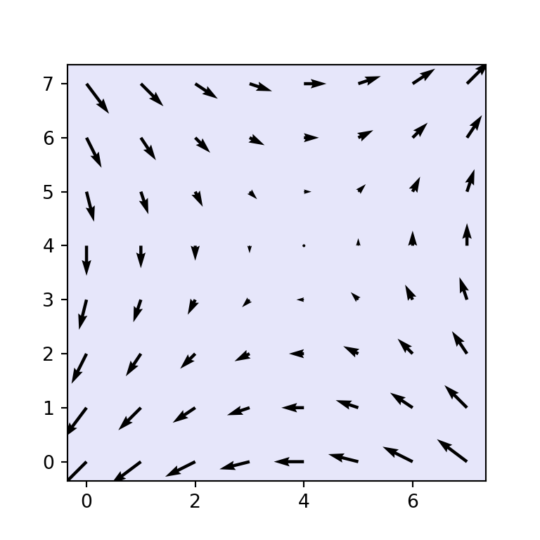

Border color

In case you want to customize the border color of the graph you will need to set a color for each of the sides of the box. You can set colors one by one or use a for loop to set all borders at once as in the example below.

import numpy as np import matplotlib.pyplot as plt fig, ax = plt.subplots() X, Y = np.mgrid[-4:4, -4:4] ax.quiver(X, Y) # Border color: for axis in ['top', 'bottom', 'left', 'right']: ax.spines[axis].set_color('red') # plt.show()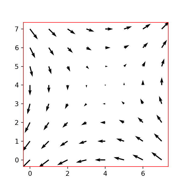

Background color of the figure

The background color of the figure can also be customized. For this purpose, you will need to set a new color to the figure ( fig ) with fig.set_facecolor , e.g. fig.set_facecolor(«aliceblue») if you want to use the aliceblue color, or just input the desired color to the facecolor argument of the subplots function, as shown below.

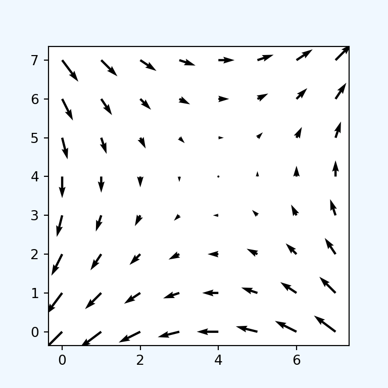
import numpy as np import matplotlib.pyplot as plt fig, ax = plt.subplots(facecolor = 'aliceblue') X, Y = np.mgrid[-4:4, -4:4] ax.quiver(X, Y) # plt.show()

Change the background colors using predefined styles

Matplotlib provides several predefined styles or themes to customize the background colors. You will need to pass the desired style name to the style.use function, as in the following example. If you want to know the names of all the available styles type print(plt.style.available) after importing matplotlib.pyplot as plt .

import numpy as np import matplotlib.pyplot as plt # Using a style plt.style.use('Solarize_Light2') fig, ax = plt.subplots() X, Y = np.mgrid[-4:4, -4:4] # Plot ax.quiver(X, Y) # plt.show()

Источник

Как изменить цвет фона в Matplotlib (с примерами)

Самый простой способ изменить цвет фона графика в Matplotlib — использовать аргумент set_facecolor() .

Если вы определяете фигуру и ось в Matplotlib, используя следующий синтаксис:

Затем вы можете просто использовать следующий синтаксис для определения цвета фона графика:

В этом руководстве представлено несколько примеров использования этой функции на практике.

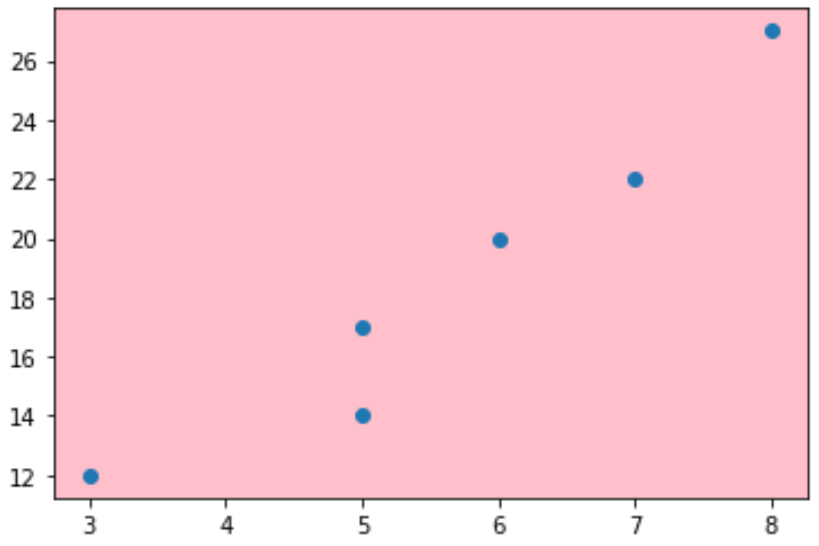
Пример 1. Установка цвета фона с использованием имени цвета

В следующем коде показано, как установить цвет фона графика Matplotlib, используя имя цвета:

import matplotlib.pyplot as plt #define plot figure and axis fig, ax = plt.subplots() #define two arrays for plotting A = [3, 5, 5, 6, 7, 8] B = [12, 14, 17, 20, 22, 27] #create scatterplot and specify background color to be pink ax.scatter (A, B) ax.set_facecolor('pink') #display scatterplot plt.show() 

Пример 2. Установка цвета фона с помощью шестнадцатеричного кода цвета

В следующем коде показано, как установить цвет фона графика Matplotlib с помощью шестнадцатеричного кода цвета:

import matplotlib.pyplot as plt #define plot figure and axis fig, ax = plt.subplots() #define two arrays for plotting A = [3, 5, 5, 6, 7, 8] B = [12, 14, 17, 20, 22, 27] #create scatterplot and specify background color to be pink ax.scatter (A, B) ax.set_facecolor('#33FFA2') #display scatterplot plt.show()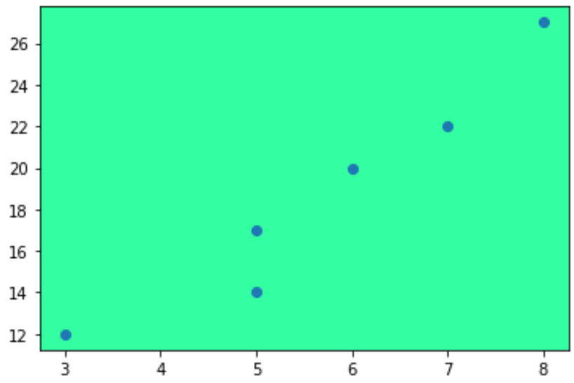 

Пример 3: установка цвета фона для определенного подграфика

Иногда у вас будет более одного графика Matplotlib. В этом случае вы можете использовать следующий код, чтобы указать цвет фона для одного графика:

import matplotlib.pyplot as plt #define subplots fig, ax = plt.subplots(2, 2) fig. tight_layout () #define background color to use for each subplot ax[0,0].set_facecolor('blue') ax[0,1].set_facecolor('pink') ax[1,0].set_facecolor('green') ax[1,1].set_facecolor('red') #display subplots plt.show() 

Источник

How to change background color in Matplotlib with Python

Actually, we are going to change the background color of any graph or figure in matplotlib with python. We have to first understand how this work, as there is a method to change the background color of any figure or graph named as “ set_facecolor “.

Changing the background color of the graph in Matplotlib with Python

Let’s understand with some examples:-

• In 1 st example, we simply draw the graph with the default background color(White).
• And in 2 nd example, we draw the graph and change the background color to Grey.
• Finally, in 3 rd example, we draw the graph and change the background color to Orange.

import matplotlib.pyplot as plt import numpy as np # Creating numpy array X = np.array([1,2,3,4,5]) Y = X**2 # Setting the figure size plt.figure(figsize=(10,6)) plt.plot(X,Y) plt.show()

In the above example, the background color of the graph is default(White), so first, we need to import two python module “matplotlib” and “numpy” by writing these two lines:-

Now, we created the numpy array and stored this in a variable named X and established the relation between X and Y. Then, we set the size of figure with method “plt.figure(figsize=(10,6))” where width=10 and height=6 and then we plotted the graph by “plt.plot(X,Y)“.

import matplotlib.pyplot as plt import numpy as np # Creating the numpy array X = np.array([1,2,3,4,5]) Y = X**2 # Setting the figure size plt.figure(figsize=(10,6)) ax = plt.axes() # Setting the background color ax.set_facecolor("grey") plt.plot(X,Y) plt.show()

In this example we are doing the same thing as in the above example, the only thing we did different from the above example is using “ax.set_facecolor(“grey”)” to change the background color of graph or figure.

import matplotlib.pyplot as plt import numpy as np # Creating the numpy array X = np.array([1,2,3,4,5]) Y = X**2 # Setting the figure size plt.figure(figsize=(10,6)) ax = plt.axes() # Setting the background color ax.set_facecolor("orange") plt.plot(X,Y) plt.show()

In this example, we only changed the background color to Orange, and the rest explanation is the same as explained above.

You may also read these articles:-

Источник