Local linear regression python

Introduction to locally weighted linear regression (Loess)¶

LOESS or LOWESS are non-parametric regression methods that combine multiple regression models in a k-nearest-neighbor-based meta-model. They address situations in which the classical procedures do not perform well or cannot be effectively applied without undue labor. LOESS combines much of the simplicity of linear least squares regression with the flexibility of nonlinear regression. It does this by fitting simple models to localized subsets of the data to build up a function that describes the variation in the data, point by point.

Local regression is sometimes referred to as a memory-based procedure, because like nearest-neighbors, we need all the training data each time we wish to compute a prediction. In order to perform local regression, there are a number of choices to be made, such as how to define the weighting function, and whether to fit a linear, constant, or quadratic regression. While all of these choices make some difference, the most important choice is the number of points which are considered as being ‘local’ to point $x_0$. This can be defined as the span $s$, which is the fraction of training points which are closest to $x_0$, or the bandwidth $\tau$ in case of a bell curve kernell, or a number of other names and terms depending on the literature used.

This parameter plays a role like that of the tuning parameter $\lambda$ in smoothing splines: it controls the flexibility of the non-linear fit. The smaller the span, the more local and wiggly will be our fit; alternatively, a very large span will lead to a global fit to the data using all of the training observations.

Procedure¶

A linear function is fitted only on a local set of points delimited by a region, using weighted least squares. The weights are given by the heights of a kernel function (i.e. weighting function) giving:

• more weights to points near the target point $x_0$ whose response is being estimated
• less weight to points further away

We obtain then a fitted model that retains only the point of the model that are close to the target point $(x_0)$. The target point then moves away on the x axis and the procedure repeats for each points.

image1 = Image(filename='/Users/User/Desktop/Computer_Science/stanford_CS229/XavierNotes/images/Fig4.png') image2 = Image(filename='/Users/User/Desktop/Computer_Science/stanford_CS229/XavierNotes/images/Fig5.png') display(image1, image2) 

Источник

Locally Weighted Linear Regression in Python

Locally Weighted Linear Regression is a non−parametric method/algorithm. In Linear regression, the data should be distributed linearly whereas Locally Weighted Regression is suitable for non−linearly distributed data. Generally, in Locally Weighted Regression, points closer to the query point are given more weightage than points away from it.

Parametric and Non-Parametric Models

Parametric

Parametric models are those which simplify the function to a known form. It has a collection of parameters that summarize the data through these parameters.

These parameters are fixed in number, which means that the model already knows about these parameters and they do not depend on the data. They are also independent in nature with respect to the training samples.

As an example, let us have a mapping function as described below.

From the equation, b0, b1, and b2 are the coefficients of the line that controls the intercept and slope. Input variables are represented by x1 and x2.

Non — Parametric

Non−parametric algorithms do not make particular assumptions about the kind of mapping function. These algorithms do not accept a specific form of the mapping function between input and output data as true.

They have the freedom to choose any functional form from the training data. As a result, for parametric models to estimate the mapping function they require much more data than parametric ones.

Derivation of Cost Function and weights

The cost function of linear regression is

In case of Locally Weighted Linear Regression, the cost function is modified to

where 𝑤(𝑖) denotes the weight of i th training sample.

The weighting function can be defined as

x is the point where we want to make the prediction. x(i) is the i th training example

τ can be called as the bandwidth of the Gaussian bell−shaped curve of the weighing function.

The value of τ can be adjusted to vary the values of w based on distance from the query point.

A small value for τ means smaller distance of the data point to the query point where value of w becomes large (more weightage) and vice versa.

The Value of w Typically Ranges From 0 to 1.

The locally Weighted Regression algorithm does not have a training phase. All weights, 𝜃 are determined during the prediction phase.

Example

Let us consider a dataset consisting of the following points:

Taking a query point as x = 7 and three points from the dataset 5,10,26

Therefore x(1) = 5, x(2) = 10 , x(3) = 26 . Let 𝜏 = 0.5

From the above examples it is evident that, the closer the query point (x) to the a particular data point/sample x(1),x(2),x(3) . etc. the larger is the value for w. The weightage decreases / falls exponentially for data points far away from the query point.

As the distance between x(i) and x increases, weights decrease. This decreases the contribution of error term to the cost function and vice versa.

Implementation in Python

The below snippet demonstrates a Locally weighted Linear Regression Algorithm.

The tips dataset can be downloaded from here

Example

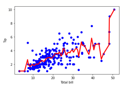
import pandas as pd import numpy as np import matplotlib.pyplot as plt %matplotlib inline df = pd.read_csv('/content/tips.csv') features = np.array(df.total_bill) labels = np.array(df.tip) def kernel(data, point, xmat, k): m,n = np.shape(xmat) ws = np.mat(np.eye((m))) for j in range(m): diff = point - data[j] ws[j,j] = np.exp(diff*diff.T/(-2.0*k**2)) return ws def local_weight(data, point, xmat, ymat, k): wei = kernel(data, point, xmat, k) return (data.T*(wei*data)).I*(data.T*(wei*ymat.T)) def local_weight_regression(xmat, ymat, k): m,n = np.shape(xmat) ypred = np.zeros(m) for i in range(m): ypred[i] = xmat[i]*local_weight(xmat, xmat[i],xmat,ymat,k) return ypred m = features.shape[0] mtip = np.mat(labels) data = np.hstack((np.ones((m, 1)), np.mat(features).T)) ypred = local_weight_regression(data, mtip, 0.5) indices = data[:,1].argsort(0) xsort = data[indices][:,0] fig = plt.figure() ax = fig.add_subplot(1,1,1) ax.scatter(features, labels, color='blue') ax.plot(xsort[:,1],ypred[indices], color = 'red', linewidth=3) plt.xlabel('Total bill') plt.ylabel('Tip') plt.show() 

Output

When can we use Locally weighted Linear Regression?

Advantage of Locally weighted Linear Regression.

• In Locally Weighted Linear Regression, local weights are calculated in relation to each datapoint so there are fewer chances of large errors.
• We fit a curved line as a result, the errors are minimized.
• In this algorithm, there are many small local functions rather than one global function which is to be minimized. Local functions are more effective in adjusting variation and errors.

Disadvantages of Locally weighted Linear Regression.

• This process is highly exhaustive and may consume a huge amount of resources.
• We may simply avoid the Locally Weighted algorithm for linearly related problems which are simpler.
• Cannot accommodate a large number of features.

Conclusion

So, in brief, a Locally weighted Linear Regression is more suited to situations where we have a nonlinear distribution of data and we still want to fit the data with a regression model without compromising on the quality of predictions.

Источник

Locally Weighted Linear Regression in Python

In this tutorial, we will discuss a special form of linear regression – locally weighted linear regression in Python. We will go through the simple Linear Regression concepts at first, and then advance onto locally weighted linear regression concepts. Finally, we will see how to code this particular algorithm in Python.

Simple Linear Regression

Linear Regression is one of the most popular and basic algorithms of Machine Learning. It is used to predict numerical data. It depicts a relationship between a dependent variable (generally called as ‘x’) on an independent variable ( generally called as ‘y’). The general equation for Linear Regression is,

Why we need Locally Weighted Linear Regression?

Linear Regression works accurately only on data has a linear relationship between them. In cases where the independent variable is not linearly related to the dependent variable we cannot use simple Linear Regression, hence we resort to Locally Weighted Linear Regression (LWLR).

Locally Weighted Linear Regression Principle

It is a very simple algorithm with only a few modifications from Linear Regression. The algorithm is as follows :

• assign different weights to the training data
• assign bigger weights to the data points that are closer to the data we are trying to predict

In LWLR, we do not split the dataset into training and test data. We use the entire dataset at once and hence this takes a lot of time, space and computational exercise.

Kernel Smoothing

We use Kernel Smoothing to find out the weights to be assigned to the training data. This is much like the Gaussian Kernel but offers a “bell-shaped kernel”. It uses the following formula :

• We find a weight matrix for each training input X. The weight matrix is always a diagonal matrix.
• The weight decreases as the distance between the predicting data and the training data.

Predicting the Results

We use the following formula to find out the values of the dependent variables :

LWLR in Python

import numpy as np import pandas as pd import matplotlib.pyplot as plt # kernel smoothing function def kernel(point, xmat, k): m,n = np.shape(xmat) weights = np.mat(np.eye((m))) for j in range(m): diff = point - X[j] weights[j, j] = np.exp(diff * diff.T / (-2.0 * k**2)) return weights # function to return local weight of eah traiining example def localWeight(point, xmat, ymat, k): wt = kernel(point, xmat, k) W = (X.T * (wt*X)).I * (X.T * wt * ymat.T) return W # root function that drives the algorithm def localWeightRegression(xmat, ymat, k): m,n = np.shape(xmat) ypred = np.zeros(m) for i in range(m): ypred[i] = xmat[i] * localWeight(xmat[i], xmat, ymat, k) return ypred #import data data = pd.read_csv('tips.csv') # place them in suitable data types colA = np.array(data.total_bill) colB = np.array(data.tip) mcolA = np.mat(colA) mcolB = np.mat(colB) m = np.shape(mcolB)[1] one = np.ones((1, m), dtype = int) # horizontal stacking X = np.hstack((one.T, mcolA.T)) print(X.shape) # predicting values using LWLR ypred = localWeightRegression(X, mcolB, 0.8) # plotting the predicted graph xsort = X.copy() xsort.sort(axis=0) plt.scatter(colA, colB, color='blue') plt.plot(xsort[:, 1], ypred[X[:, 1].argsort(0)], color='yellow', linewidth=5) plt.xlabel('Total Bill') plt.ylabel('Tip') plt.show()

Please follow the following link to see the entire code :

The results for the tips.csv dataset is :

This is a very simple method of using LWLR in Python.

Note: This algorithm gives accurate results only when non-linear relationships exist between dependent and independent variables.

Источник