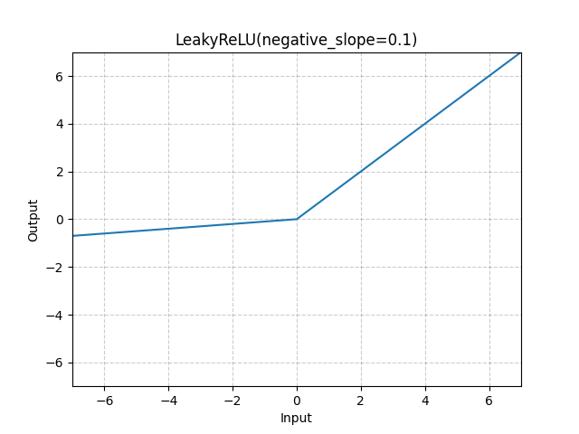
LeakyReLU layer
It allows a small gradient when the unit is not active:
>>> layer = tf.keras.layers.LeakyReLU() >>> output = layer([-3.0, -1.0, 0.0, 2.0]) >>> list(output.numpy()) [-0.9, -0.3, 0.0, 2.0] >>> layer = tf.keras.layers.LeakyReLU(alpha=0.1) >>> output = layer([-3.0, -1.0, 0.0, 2.0]) >>> list(output.numpy()) [-0.3, -0.1, 0.0, 2.0] Input shape
Arbitrary. Use the keyword argument input_shape (tuple of integers, does not include the batch axis) when using this layer as the first layer in a model.
Output shape
Функция активации ReLu в Python
Функция активации Relu в Python или Rectified Linear Activation является наиболее распространенным выбором функции активации в мире глубокого обучения. Relu обеспечивает самые современные результаты и в то же время очень эффективен с точки зрения вычислений.
Основная концепция функции активации Relu заключается в следующем:
Return 0 if the input is negative otherwise return the input as it is.
Мы можем представить это математически следующим образом:

Псевдокод для Relu следующий:
if input > 0: return input else: return 0
В этом руководстве мы узнаем, как реализовать нашу собственную функцию ReLu, узнаем о некоторых ее недостатках и узнаем о лучшей версии.
Реализация функции ReLu
Напишем собственную реализацию Relu на Python. Мы будем использовать встроенную функцию max для ее реализации.
Чтобы протестировать функцию, запустим ее на нескольких входах.
x = 1.0 print('Applying Relu on (%.1f) gives %.1f' % (x, relu(x))) x = -10.0 print('Applying Relu on (%.1f) gives %.1f' % (x, relu(x))) x = 0.0 print('Applying Relu on (%.1f) gives %.1f' % (x, relu(x))) x = 15.0 print('Applying Relu on (%.1f) gives %.1f' % (x, relu(x))) x = -20.0 print('Applying Relu on (%.1f) gives %.1f' % (x, relu(x))) Полный код
def relu(x): return max(0.0, x) x = 1.0 print('Applying Relu on (%.1f) gives %.1f' % (x, relu(x))) x = -10.0 print('Applying Relu on (%.1f) gives %.1f' % (x, relu(x))) x = 0.0 print('Applying Relu on (%.1f) gives %.1f' % (x, relu(x))) x = 15.0 print('Applying Relu on (%.1f) gives %.1f' % (x, relu(x))) x = -20.0 print('Applying Relu on (%.1f) gives %.1f' % (x, relu(x))) Applying Relu on (1.0) gives 1.0 Applying Relu on (-10.0) gives 0.0 Applying Relu on (0.0) gives 0.0 Applying Relu on (15.0) gives 15.0 Applying Relu on (-20.0) gives 0.0
Производная ReLu
Посмотрим, каким будет градиент (производная) функции ReLu. При дифференцировании получим следующую функцию:
Мы видим, что для значений x меньше нуля градиент равен 0. Это означает, что веса и смещения для некоторых нейронов не обновляются. Это может быть проблемой в тренировочном процессе.
Чтобы решить эту проблему, у нас есть функция Leaky ReLu.
Функция Leaky ReLu
Функция Leaky ReLu – это импровизация обычной функции ReLu. Чтобы решить проблему нулевого градиента для отрицательного значения, Leaky ReLu дает чрезвычайно малую линейную составляющую x отрицательным входам.
Математически мы можем выразить Leaky ReLu как:
Здесь a – небольшая константа, подобная 0,01, которую мы взяли выше.
Графически это можно представить как:

Градиент Leaky ReLu
Рассчитаем градиент для функции Leaky ReLu. Градиент может быть таким:
В этом случае градиент для отрицательных входов не равен нулю. Это значит, что обновится весь нейрон.
Реализация Leaky ReLu
Реализация Leaky ReLu приведена ниже:
def relu(x): if x>0 : return x else : return 0.01*x
Давайте попробуем это на месте.
x = 1.0 print('Applying Leaky Relu on (%.1f) gives %.1f' % (x, leaky_relu(x))) x = -10.0 print('Applying Leaky Relu on (%.1f) gives %.1f' % (x, leaky_relu(x))) x = 0.0 print('Applying Leaky Relu on (%.1f) gives %.1f' % (x, leaky_relu(x))) x = 15.0 print('Applying Leaky Relu on (%.1f) gives %.1f' % (x, leaky_relu(x))) x = -20.0 print('Applying Leaky Relu on (%.1f) gives %.1f' % (x, leaky_relu(x))) Полный код
Полный код Leaky ReLu приведен ниже:
def leaky_relu(x): if x>0 : return x else : return 0.01*x x = 1.0 print('Applying Leaky Relu on (%.1f) gives %.1f' % (x, leaky_relu(x))) x = -10.0 print('Applying Leaky Relu on (%.1f) gives %.1f' % (x, leaky_relu(x))) x = 0.0 print('Applying Leaky Relu on (%.1f) gives %.1f' % (x, leaky_relu(x))) x = 15.0 print('Applying Leaky Relu on (%.1f) gives %.1f' % (x, leaky_relu(x))) x = -20.0 print('Applying Leaky Relu on (%.1f) gives %.1f' % (x, leaky_relu(x))) Applying Leaky Relu on (1.0) gives 1.0 Applying Leaky Relu on (-10.0) gives -0.1 Applying Leaky Relu on (0.0) gives 0.0 Applying Leaky Relu on (15.0) gives 15.0 Applying Leaky Relu on (-20.0) gives -0.2
Заключение
Это руководство было посвящено функции ReLu в Python. Мы также увидели улучшенную версию функции Leaky ReLu, которая решает проблему нулевых градиентов для отрицательных значений.
LeakyReLU
Parameters :
- negative_slope (float) – Controls the angle of the negative slope (which is used for negative input values). Default: 1e-2
- inplace (bool) – can optionally do the operation in-place. Default: False
Shape:
- Input: ( ∗ ) (*) ( ∗ ) where * means, any number of additional dimensions
- Output: ( ∗ ) (*) ( ∗ ) , same shape as the input
>>> m = nn.LeakyReLU(0.1) >>> input = torch.randn(2) >>> output = m(input)
© Copyright 2023, PyTorch Contributors.
Docs
Access comprehensive developer documentation for PyTorch
Tutorials
Get in-depth tutorials for beginners and advanced developers
Resources
Find development resources and get your questions answered
© Copyright The Linux Foundation. The PyTorch Foundation is a project of The Linux Foundation. For web site terms of use, trademark policy and other policies applicable to The PyTorch Foundation please see www.linuxfoundation.org/policies/. The PyTorch Foundation supports the PyTorch open source project, which has been established as PyTorch Project a Series of LF Projects, LLC. For policies applicable to the PyTorch Project a Series of LF Projects, LLC, please see www.lfprojects.org/policies/.
To analyze traffic and optimize your experience, we serve cookies on this site. By clicking or navigating, you agree to allow our usage of cookies. As the current maintainers of this site, Facebook’s Cookies Policy applies. Learn more, including about available controls: Cookies Policy.
Activation Functions

When building your Deep Learning model, activation functions are an important choice to make. In this article, we’ll review the main activation functions, their implementations in Python, and advantages/disadvantages of each.
Linear Activation
Linear activation is the simplest form of activation. In that case, \(f(x)\) is just the identity. If you use a linear activation function the wrong way, your whole Neural Network ends up being a regression :
\[\hat = \sigma(h) = h = W^ h_1 = W^ W^ X = W’ X\]
Linear activations are only needed when you’re considering a regression problem, as a last layer. The whole idea behind the other activation functions is to create non-linearity, to be able to model highly non-linear data that cannot be solved by a simple regression !
ReLU
ReLU stands for Rectified Linear Unit. It is a widely used activation function. The formula is simply the maximum between \(x\) and 0 :
To implement this in Python, you might simply use :
The derivative of the ReLU is :
def der_relu(x): if x 0 : return 0 if x > 0 : return 1 Let’s simulate some data and plot them to illustrate this activation function :
import numpy as np import matplotlib.pyplot as plt # Data which will go through activations x = np.linspace(-10,10,100) plt.figure(figsize=(12,8)) plt.plot(x, list(map(lambda x: relu(x),x)), label="relu") plt.plot(x, list(map(lambda x: der_relu(x),x)), label="derivative") plt.title("ReLU") plt.legend() plt.show() 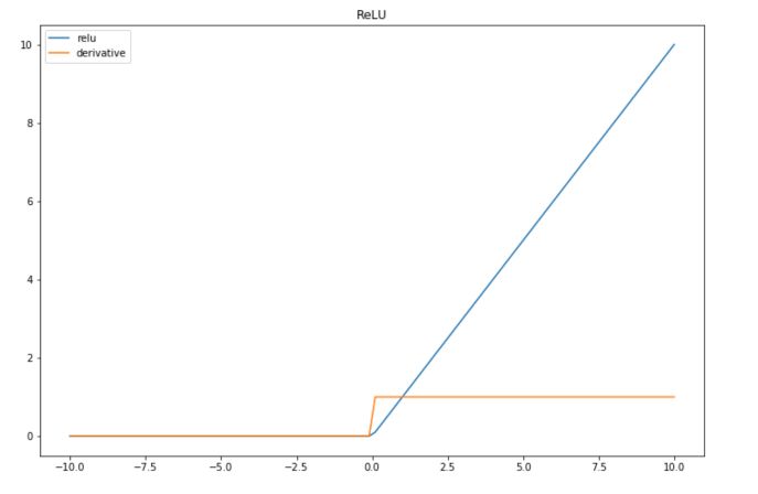
| Advantage | Easy to implement and quick to compute |
| Disadvantage | Problematic when we have lots of negative values, since the outcome is always 0 and leads to the death of the neuron |
Leaky-ReLU
Leaky-ReLU is an improvement of the main default of the ReLU, in the sense that it can handle the negative values pretty well, but still brings non-linearity.
The derivative is also simple to compute :
def leaky_relu(x): return max(0.01*x,x) def der_leaky_relu(x): if x 0 : return 0.01 if x >= 0 : return 1 And we can plot the result of this activation function :
plt.figure(figsize=(12,8)) plt.plot(x, list(map(lambda x: leaky_relu(x),x)), label="leaky-relu") plt.plot(x, list(map(lambda x: der_leaky_relu(x),x)), label="derivative") plt.title("Leaky-ReLU") plt.legend() plt.show() 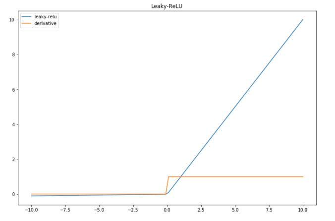
| Advantage | Leaky-ReLU overcomes the problem of the death of the neuron linked to a zero-slope. |
| Disadvantage | The factor 0.01 is arbitraty, and can be tuned (PReLU for parametric ReLU) |
Exponential Linear Units (ELU) try to make the mean activations closer to zero, which speeds up learning.
\(f(x) = x\) if \(x>0\), and \(a(e^x -1)\) otherwise, where \(a\) is a positive constant.
def elu(x): if x > 0 : return x else : return (np.exp(x)-1) def der_elu(x): if x > 0 : return 1 else : return np.exp(x) plt.figure(figsize=(12,8)) plt.plot(x, list(map(lambda x: elu(x),x)), label="elu") plt.plot(x, list(map(lambda x: der_elu(x),x)), label="derivative") plt.title("ELU") plt.legend() plt.show() 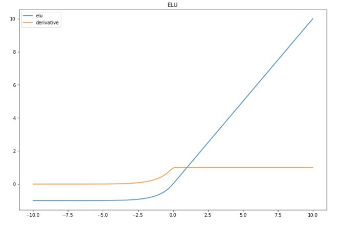
| Advantage | Can achieve higher accuracy than ReLU |
| Disadvantage | Same as ReLU, and a needs to be tuned |
Softplus
The Softplus function is a continuous approximation of ReLU. It is given by :
The derivative of the softplus function is :
You can implement them in Python :
def softplus(x): return np.log(1+np.exp(x)) def der_softplus(x): return 1/(1+np.exp(x))*np.exp(x) plt.figure(figsize=(12,8)) plt.plot(x, list(map(lambda x: softplus(x),x)), label="softplus") plt.plot(x, list(map(lambda x: der_softplus(x),x)), label="derivative") plt.title("Softplus") plt.legend() plt.show() 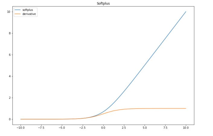
| Advantage | Softplus is continuous and might have good properties in terms of derivability. It is interesting to use it when the values are between 0 and 1. |
| Disadvantage | As ReLU, problematic when we have lots of negative values, since the outcome gets really close to 0 and might lead to the death of the neuron |
Sigmoid
Sigmoid is one of the most common activation functions in litterature these days. The sigmoid function has the following form :
The derivative of the sigmoid is :
def softmax(x): return 1/(1+np.exp(-x)) def der_softmax(x): return 1/(1+np.exp(-x)) * (1-1/(1+np.exp(-x))) plt.figure(figsize=(12,8)) plt.plot(x, list(map(lambda x: softmax(x),x)), label="softmax") plt.plot(x, list(map(lambda x: der_softmax(x),x)), label="derivative") plt.title("Softmax") plt.legend() plt.show() 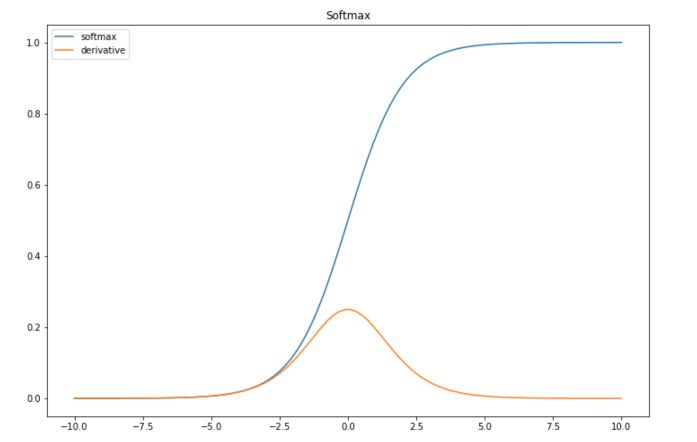
It might not be obvious when considering data between \(-10\) and \(10\) only, but the sigmoid is subject to the vanishing gradient problem. This means that the gradient will tend to vanish as \(x\) takes large values.
Since the gradient is the sigmoid times 1 minus the sigmoid, the gradient can be efficiently computed. If we keep track of the sigmoids, we can compute the gradient really quickly.
| Advantage | Interpretability of the output mapped between 0 and 1, compute gradient quickly |
| Disadvantage | Vanishing Gradient |
Hyperbolic Tangent
Hyperbolic tangent is quite similar to the sigmoid function, expect is maps the input between -1 and 1.
The derivative is computed in the following way :
def hyperb(x): return (np.exp(x)-np.exp(-x)) / (np.exp(x) + np.exp(-x)) def der_hyperb(x): return 1 - ((np.exp(x)-np.exp(-x)) / (np.exp(x) + np.exp(-x)))**2 plt.figure(figsize=(12,8)) plt.plot(x, list(map(lambda x: hyperb(x),x)), label="hyperbolic") plt.plot(x, list(map(lambda x: der_hyperb(x),x)), label="derivative") plt.title("Hyperbolic") plt.legend() plt.show() 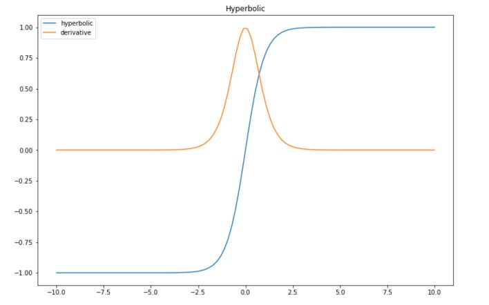
| Advantage | Efficient since it has mean 0 in the middle layers between -1 and 1 |
| Disadvantage | Vanishing gradient too |
Arctan
This activation function maps the input values in the range \((− \pi / 2, \pi / 2)\). It is the inverse of a hyperbolic tangent function.
def arctan(x): return np.arctan(x) def der_arctan(x): return 1 / (1+x**2) plt.figure(figsize=(12,8)) plt.plot(x, list(map(lambda x: arctan(x),x)), label="arctan") plt.plot(x, list(map(lambda x: der_arctan(x),x)), label="derivative") plt.title("Arctan") plt.legend() plt.show() 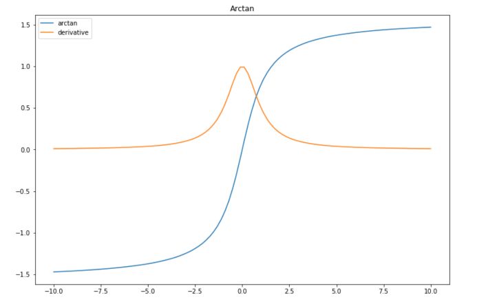
| Advantage | Simple derivative |
| Disadvantage | Vanishing gradient |