Способы создания гистограмм с помощью Python
За последний год я сталкивалась с необходимостью рисования гистограмм и столбчатых диаграмм достаточно часто для того, чтобы появилось желание и возможность об этом написать. Кроме того, мне самой довольно сильно не хватало подобной информации. В этой статье приведен обзор 3 методов создания таких графиков на языке Python.
Начнем с того, чего я сама по своей неопытности не знала очень долго: столбчатые диаграммы и гистограммы — разные вещи. Основное отличие состоит в том, что гистограмма показывает частотное распределение — мы задаем набор значений оси Ox, а по Oy всегда откладывается частота. В столбчатой диаграмме (которую в англоязычной литературе уместно было бы назвать barplot) мы задаем и значения оси абсцисс, и значения оси ординат.
Для демонстрации я буду использовать избитый набор данных библиотеки scikit learn Iris. Начнем c импортов:
import pandas as pd import numpy as np import matplotlib import matplotlib.pyplot as plt from sklearn import datasets iris = datasets.load_iris() Преобразуем набор данных iris в dataframe — так нам удобнее будет с ним работать в будущем.
data = pd.DataFrame(data= np.c_[iris['data'], iris['target']], columns= iris['feature_names'] + ['target']) Из интересующих нас параметров data содержит информацию о длине чашелистиков и лепестков и ширине чашелистиков и лепестков.
Используем Matplotlib
Построение гистограммы
Cтроим обычную гистограмму, показывающую частотное распределение длин лепестков и чашелистиков:
fig, axs = plt.subplots(1, 2) n_bins = len(data) axs[0].hist(data['sepal length (cm)'], bins=n_bins) axs[0].set_title('sepal length') axs[1].hist(data['petal length (cm)'], bins=n_bins) axs[1].set_title('petal length') 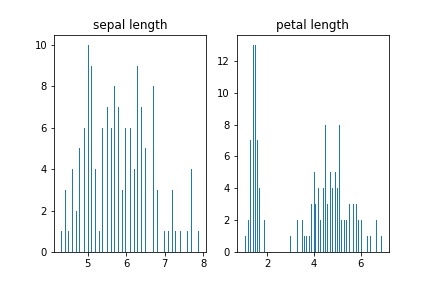
Построение столбчатой диаграммы
Используем методы matplotlib-а, чтобы сравнить ширину листьев и чашелистиков. Это кажется удобнее всего делать на одном графике:
x = np.arange(len(data[:50])) width = 0.35 Для примера и в целях упрощения картинки возьмем первые 50 строк dataframe.
fig, ax = plt.subplots(figsize=(40,5)) rects1 = ax.bar(x - width/2, data['sepal width (cm)'][:50], width, label='sepal width') rects2 = ax.bar(x + width/2, data['petal width (cm)'][:50], width, label='petal width') ax.set_ylabel('cm') ax.set_xticks(x) ax.legend()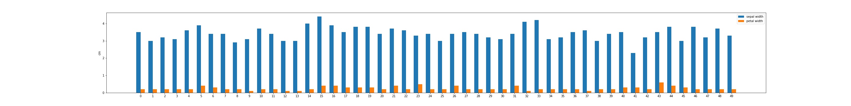
Используем методы seaborn
На мой взгляд, многие задачи по построению гистограмм проще и эффективнее выполнять с помощью методов seaborn (кроме того, seaborn выигрывает еще и своими графическими возможностями, на мой взгляд).
Я приведу пример задач, решающихся в seaborn с помощью одной строчки кода. Особенно seaborn выигрышный, когда надо построить распределение. Скажем, нам надо построить распределение длин чашелистиков. Решение этой задачи таково:
sns_plot = sns.distplot(data['sepal width (cm)']) fig = sns_plot.get_figure() 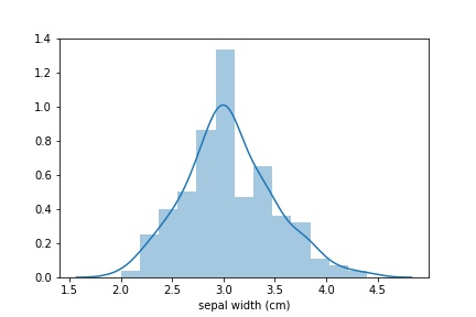
Если же вам необходим только график распределения, сделать его можно так:
snsplot = sns.kdeplot(data['sepal width (cm)'], shade=True) fig = snsplot.get_figure() 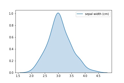
Подробнее о построении распределений в seaborn можно почитать тут.
Здесь все просто. На самом деле, это оболочка matplotlib.pyplot.hist(), но вызов функции через pd.hist() иногда удобнее менее поворотливых конструкций matplotlib-a. В документации библиотеки pandas можно прочитать больше.
h = data['petal width (cm)'].hist() fig = h.get_figure() Спасибо, что прочитали до конца! Буду рада отзывам и комментариям!
Histograms#
To generate a 1D histogram we only need a single vector of numbers. For a 2D histogram we’ll need a second vector. We’ll generate both below, and show the histogram for each vector.
N_points = 100000 n_bins = 20 # Generate two normal distributions dist1 = rng.standard_normal(N_points) dist2 = 0.4 * rng.standard_normal(N_points) + 5 fig, axs = plt.subplots(1, 2, sharey=True, tight_layout=True) # We can set the number of bins with the *bins* keyword argument. axs[0].hist(dist1, bins=n_bins) axs[1].hist(dist2, bins=n_bins)

Updating histogram colors#
The histogram method returns (among other things) a patches object. This gives us access to the properties of the objects drawn. Using this, we can edit the histogram to our liking. Let’s change the color of each bar based on its y value.
fig, axs = plt.subplots(1, 2, tight_layout=True) # N is the count in each bin, bins is the lower-limit of the bin N, bins, patches = axs[0].hist(dist1, bins=n_bins) # We'll color code by height, but you could use any scalar fracs = N / N.max() # we need to normalize the data to 0..1 for the full range of the colormap norm = colors.Normalize(fracs.min(), fracs.max()) # Now, we'll loop through our objects and set the color of each accordingly for thisfrac, thispatch in zip(fracs, patches): color = plt.cm.viridis(norm(thisfrac)) thispatch.set_facecolor(color) # We can also normalize our inputs by the total number of counts axs[1].hist(dist1, bins=n_bins, density=True) # Now we format the y-axis to display percentage axs[1].yaxis.set_major_formatter(PercentFormatter(xmax=1))

Plot a 2D histogram#
To plot a 2D histogram, one only needs two vectors of the same length, corresponding to each axis of the histogram.
fig, ax = plt.subplots(tight_layout=True) hist = ax.hist2d(dist1, dist2)

Customizing your histogram#
Customizing a 2D histogram is similar to the 1D case, you can control visual components such as the bin size or color normalization.
fig, axs = plt.subplots(3, 1, figsize=(5, 15), sharex=True, sharey=True, tight_layout=True) # We can increase the number of bins on each axis axs[0].hist2d(dist1, dist2, bins=40) # As well as define normalization of the colors axs[1].hist2d(dist1, dist2, bins=40, norm=colors.LogNorm()) # We can also define custom numbers of bins for each axis axs[2].hist2d(dist1, dist2, bins=(80, 10), norm=colors.LogNorm()) plt.show()

The use of the following functions, methods, classes and modules is shown in this example:
Total running time of the script: ( 0 minutes 2.265 seconds)
matplotlib.pyplot.hist#
matplotlib.pyplot. hist ( x , bins = None , range = None , density = False , weights = None , cumulative = False , bottom = None , histtype = ‘bar’ , align = ‘mid’ , orientation = ‘vertical’ , rwidth = None , log = False , color = None , label = None , stacked = False , * , data = None , ** kwargs ) [source] #
Compute and plot a histogram.
This method uses numpy.histogram to bin the data in x and count the number of values in each bin, then draws the distribution either as a BarContainer or Polygon . The bins, range, density, and weights parameters are forwarded to numpy.histogram .
If the data has already been binned and counted, use bar or stairs to plot the distribution:
counts, bins = np.histogram(x) plt.stairs(counts, bins)
Alternatively, plot pre-computed bins and counts using hist() by treating each bin as a single point with a weight equal to its count:
plt.hist(bins[:-1], bins, weights=counts)
The data input x can be a singular array, a list of datasets of potentially different lengths ([x0, x1, . ]), or a 2D ndarray in which each column is a dataset. Note that the ndarray form is transposed relative to the list form. If the input is an array, then the return value is a tuple (n, bins, patches); if the input is a sequence of arrays, then the return value is a tuple ([n0, n1, . ], bins, [patches0, patches1, . ]).
Masked arrays are not supported.
Parameters : x (n,) array or sequence of (n,) arrays
Input values, this takes either a single array or a sequence of arrays which are not required to be of the same length.
bins int or sequence or str, default: rcParams[«hist.bins»] (default: 10 )
If bins is an integer, it defines the number of equal-width bins in the range.
If bins is a sequence, it defines the bin edges, including the left edge of the first bin and the right edge of the last bin; in this case, bins may be unequally spaced. All but the last (righthand-most) bin is half-open. In other words, if bins is:
then the first bin is [1, 2) (including 1, but excluding 2) and the second [2, 3) . The last bin, however, is [3, 4] , which includes 4.
If bins is a string, it is one of the binning strategies supported by numpy.histogram_bin_edges : ‘auto’, ‘fd’, ‘doane’, ‘scott’, ‘stone’, ‘rice’, ‘sturges’, or ‘sqrt’.
range tuple or None, default: None
The lower and upper range of the bins. Lower and upper outliers are ignored. If not provided, range is (x.min(), x.max()) . Range has no effect if bins is a sequence.
If bins is a sequence or range is specified, autoscaling is based on the specified bin range instead of the range of x.
density bool, default: False
If True , draw and return a probability density: each bin will display the bin’s raw count divided by the total number of counts and the bin width ( density = counts / (sum(counts) * np.diff(bins)) ), so that the area under the histogram integrates to 1 ( np.sum(density * np.diff(bins)) == 1 ).
If stacked is also True , the sum of the histograms is normalized to 1.
weights (n,) array-like or None, default: None
An array of weights, of the same shape as x. Each value in x only contributes its associated weight towards the bin count (instead of 1). If density is True , the weights are normalized, so that the integral of the density over the range remains 1.
cumulative bool or -1, default: False
If True , then a histogram is computed where each bin gives the counts in that bin plus all bins for smaller values. The last bin gives the total number of datapoints.
If density is also True then the histogram is normalized such that the last bin equals 1.
If cumulative is a number less than 0 (e.g., -1), the direction of accumulation is reversed. In this case, if density is also True , then the histogram is normalized such that the first bin equals 1.
bottom array-like, scalar, or None, default: None
Location of the bottom of each bin, i.e. bins are drawn from bottom to bottom + hist(x, bins) If a scalar, the bottom of each bin is shifted by the same amount. If an array, each bin is shifted independently and the length of bottom must match the number of bins. If None, defaults to 0.
The type of histogram to draw.
- ‘bar’ is a traditional bar-type histogram. If multiple data are given the bars are arranged side by side.
- ‘barstacked’ is a bar-type histogram where multiple data are stacked on top of each other.
- ‘step’ generates a lineplot that is by default unfilled.
- ‘stepfilled’ generates a lineplot that is by default filled.
The horizontal alignment of the histogram bars.
- ‘left’: bars are centered on the left bin edges.
- ‘mid’: bars are centered between the bin edges.
- ‘right’: bars are centered on the right bin edges.
If ‘horizontal’, barh will be used for bar-type histograms and the bottom kwarg will be the left edges.
rwidth float or None, default: None
The relative width of the bars as a fraction of the bin width. If None , automatically compute the width.
Ignored if histtype is ‘step’ or ‘stepfilled’.
log bool, default: False
If True , the histogram axis will be set to a log scale.
color color or array-like of colors or None, default: None
Color or sequence of colors, one per dataset. Default ( None ) uses the standard line color sequence.
label str or None, default: None
String, or sequence of strings to match multiple datasets. Bar charts yield multiple patches per dataset, but only the first gets the label, so that legend will work as expected.
stacked bool, default: False
If True , multiple data are stacked on top of each other If False multiple data are arranged side by side if histtype is ‘bar’ or on top of each other if histtype is ‘step’
Returns : n array or list of arrays
The values of the histogram bins. See density and weights for a description of the possible semantics. If input x is an array, then this is an array of length nbins. If input is a sequence of arrays [data1, data2, . ] , then this is a list of arrays with the values of the histograms for each of the arrays in the same order. The dtype of the array n (or of its element arrays) will always be float even if no weighting or normalization is used.
bins array
The edges of the bins. Length nbins + 1 (nbins left edges and right edge of last bin). Always a single array even when multiple data sets are passed in.
patches BarContainer or list of a single Polygon or list of such objects
Container of individual artists used to create the histogram or list of such containers if there are multiple input datasets.
Other Parameters : data indexable object, optional
If given, the following parameters also accept a string s , which is interpreted as data[s] (unless this raises an exception):
2D histogram with rectangular bins
2D histogram with hexagonal bins
Plot a pre-computed histogram
Plot a pre-computed histogram
For large numbers of bins (>1000), plotting can be significantly accelerated by using stairs to plot a pre-computed histogram ( plt.stairs(*np.histogram(data)) ), or by setting histtype to ‘step’ or ‘stepfilled’ rather than ‘bar’ or ‘barstacked’.