Gradient descent implementation python

Содержание

What is gradient descent ?
Example by hand :
Gradient descent in Python :
How to implement a gradient descent in Python to find a local minimum ?
Algorithm for Gradient Descent
Partial Derivatives (Gradients)
Parameter Updation

What is gradient descent ?

It is an optimization algorithm to find the minimum of a function. We start with a random point on the function and move in the negative direction of the gradient of the function to reach the local/global minima.

Example by hand :

Question : Find the local minima of the function y=(x+5)² starting from the point x=3

Solution : We know the answer just by looking at the graph. y = (x+5)² reaches it’s minimum value when x = -5 (i.e when x=-5, y=0). Hence x=-5 is the local and global minima of the function.

Now, let’s see how to obtain the same numerically using gradient descent.

Step 1 : Initialize x =3. Then, find the gradient of the function, dy/dx = 2*(x+5).

Step 2 : Move in the direction of the negative of the gradient (Why?). But wait, how much to move? For that, we require a learning rate. Let us assume the learning rate → 0.01

Step 3 : Let’s perform 2 iterations of gradient descent

Step 4 : We can observe that the X value is slowly decreasing and should converge to -5 (the local minima). However, how many iterations should we perform?

Let us set a precision variable in our algorithm which calculates the difference between two consecutive “x” values . If the difference between x values from 2 consecutive iterations is lesser than the precision we set, stop the algorithm !

Gradient descent in Python :

Step 1 : Initialize parameters

cur_x = 3 # The algorithm starts at x=3
rate = 0.01 # Learning rate
precision = 0.000001 #This tells us when to stop the algorithm
previous_step_size = 1 #
max_iters = 10000 # maximum number of iterations
iters = 0 #iteration counter
df = lambda x: 2*(x+5) #Gradient of our function

Step 2 : Run a loop to perform gradient descent :

i. Stop loop when difference between x values from 2 consecutive iterations is less than 0.000001 or when number of iterations exceeds 10,000

while previous_step_size > precision and iters < max_iters:
prev_x = cur_x #Store current x value in prev_x 
cur_x = cur_x - rate * df(prev_x) #Grad descent 
previous_step_size = abs(cur_x - prev_x) #Change in x 
iters = iters+1 #iteration count 
print("Iteration",iters,"\nX value is",cur_x) #Print iterations 

print("The local minimum occurs at", cur_x)

Output : From the output below, we can observe the x values for the first 10 iterations- which can be cross checked with our calculation above. The algorithm runs for 595 iterations before it terminates. The code and solution is embedded below for reference.

Источник

How to implement a gradient descent in Python to find a local minimum ?

Gradient Descent is an iterative algorithm that is used to minimize a function by finding the optimal parameters. Gradient Descent can be applied to any dimension function i.e. 1-D, 2-D, 3-D. In this article, we will be working on finding global minima for parabolic function (2-D) and will be implementing gradient descent in python to find the optimal parameters for the linear regression equation (1-D). Before diving into the implementation part, let us make sure the set of parameters required to implement the gradient descent algorithm. To implement a gradient descent algorithm, we require a cost function that needs to be minimized, the number of iterations, a learning rate to determine the step size at each iteration while moving towards the minimum, partial derivatives for weight & bias to update the parameters at each iteration, and a prediction function.

Till now we have seen the parameters required for gradient descent. Now let us map the parameters with the gradient descent algorithm and work on an example to better understand gradient descent. Let us consider a parabolic equation y=4x 2 . By looking at the equation we can identify that the parabolic function is minimum at x = 0 i.e. at x=0, y=0. Therefore x=0 is the local minima of the parabolic function y=4x 2 . Now let us see the algorithm for gradient descent and how we can obtain the local minima by applying gradient descent:

Algorithm for Gradient Descent

Steps should be made in proportion to the negative of the function gradient (move away from the gradient) at the current point to find local minima. Gradient Ascent is the procedure for approaching a local maximum of a function by taking steps proportional to the positive of the gradient (moving towards the gradient).

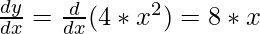
Step 1: Initializing all the necessary parameters and deriving the gradient function for the parabolic equation 4x 2 . The derivative of x 2 is 2x, so the derivative of the parabolic equation 4x 2 will be 8x.

x₀ = 3 (random initialization of x)

learning_rate = 0.01 (to determine the step size while moving towards local minima)

$\frac<dy data-lazy-src=$

gradient = =\frac(4*x^2) = 8*x » width=»» height=»»/> (Calculating the gradient function)

Step 2: Let us perform 3 iterations of gradient descent:

For each iteration keep on updating the value of x based on the gradient descent formula.

Iteration 1: x₁ = x₀ - (learning_rate * gradient) x₁ = 3 - (0.01 * (8 * 3)) x₁ = 3 - 0.24 x₁ = 2.76 Iteration 2: x₂ = x₁ - (learning_rate * gradient) x₂ = 2.76 - (0.01 * (8 * 2.76)) x₂ = 2.76 - 0.2208 x₂ = 2.5392 Iteration 3: x₃ = x₂ - (learning_rate * gradient) x₃ = 2.5392 - (0.01 * (8 * 2.5392)) x₃ = 2.5392 - 0.203136 x₃ = 2.3360

From the above three iterations of gradient descent, we can notice that the value of x is decreasing iteration by iteration and will slowly converge to 0 (local minima) by running the gradient descent for more iterations. Now you might have a question, for how many iterations we should run gradient descent?

We can set a stopping threshold i.e. when the difference between the previous and the present value of x becomes less than the stopping threshold we stop the iterations. When it comes to the implementation of gradient descent for machine learning algorithms and deep learning algorithms we try to minimize the cost function in the algorithms using gradient descent. Now that we are clear with the gradient descent’s internal working, let us look into the python implementation of gradient descent where we will be minimizing the cost function of the linear regression algorithm and finding the best fit line. In our case the parameters are below mentioned:

Prediction Function

The prediction function for the linear regression algorithm is a linear equation given by y=wx+b.

prediction_function (y) = (w * x) + b Here, x is the independent variable y is the dependent variable w is the weight associated with input variable b is the bias

Cost Function

The cost function is used to calculate the loss based on the predictions made. In linear regression, we use mean squared error to calculate the loss. Mean Squared Error is the sum of the squared differences between the actual and predicted values.

Partial Derivatives (Gradients)

Calculating the partial derivatives for weight and bias using the cost function. We get:

$\frac<dJ data-lazy-src=$

=(\frac)^x_i*(y_ — (wx_+b))>» width=»» height=»»/>

Parameter Updation

Updating the weight and bias by subtracting the multiplication of learning rates and their respective gradients.

w = w - (learning_rate * (dJ/dw)) b = b - (learning_rate * (dJ/db))

Python Implementation for Gradient Descent

In the implementation part, we will be writing two functions, one will be the cost functions that take the actual output and the predicted output as input and returns the loss, the second will be the actual gradient descent function which takes the independent variable, target variable as input and finds the best fit line using gradient descent algorithm. The iterations, learning_rate, and stopping threshold are the tuning parameters for the gradient descent algorithm and can be tuned by the user. In the main function, we will be initializing linearly related random data and applying the gradient descent algorithm on the data to find the best fit line. The optimal weight and bias found by using the gradient descent algorithm are later used to plot the best fit line in the main function. The iterations specify the number of times the update of parameters must be done, the stopping threshold is the minimum change of loss between two successive iterations to stop the gradient descent algorithm.

Источник