Conditional formatting excel python

Python Xlsxwriter Create Excel Part 4 Conditional Formatting

The Python xlsxwriter library is capable of creating all sorts of conditional formatting for our Excel file. Let’s take a look at how to do that. One of our friends on Youtube requested this, and here you go!

This is part of the automating Excel series. If you need an introduction to the xlsxwriter library that we are using, head to part 1 of the series.

Getting The Python Environment Ready

Let’s head into Python, generate some values, and a xlsxwriter workbook. Time for Christmas decoration!

The three formats we have created are format_r (red), format_y (yellow), and format_g (green).

) format_y = wb.add_format() format_g = wb.add_format()

Review Time

1. We need a workbook object (wb) and a worksheet object (ws).
2. Either the “A1” or (row, col) style notation can be used to reference cells and ranges.
3. Create Excel format by using the workbook.add_format() method.
4. Format a cell by writing data and formatting simultaneously into cell/range.

New Concept

1. To create conditional formatting , use worksheet.conditional_format(‘A1’, parameters>)
2. A conditional formatting is superimposed over the existing cell format. Not all cell format properties can be modified, such as font name, size, alignment, etc.
3. Related to #2 above, most of the time we use conditional formatting just to highlight cells. i.e. change cell color.

Xlsxwriter Conditional Formatting parameters

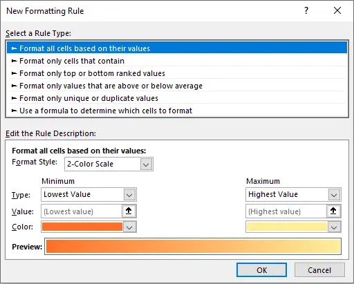
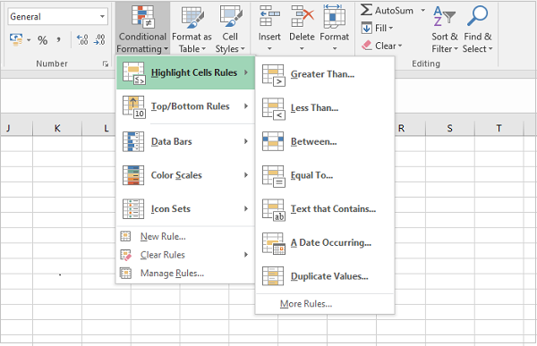
• type – are we formatting cells, numbers, text, ranking, average, duplicate or formula? See the picture below, the “type” refers to the “Rule Type”.
• criteria – do we want to find the “greater/less than”, “contain” certain text, top items, etc
• value – usually in conjuction with the criteria, “great than 7”, “between 5 and 7”, “above” average, etc
• format – the formatting, usually it’s just changing the cell/font color

Now we got the theory out of the way, let’s see how to apply them. Because we are going through several examples, so we’ll group our Python code into functions to make it more organized.

Following the order of the above screen “Rule Type” offered by Excel, we’ll take a look at each scenario below.

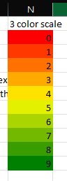
Conditional Formatting All Cells Color Scale

I hope you like rainbow . We can specify three colors (min, mid and max) and Excel will make a pretty rainbow for us. If you prefer only dual colors, then change ‘type’ to be ‘2_color_scale’ , and then simply remove the ‘mid_color’ .

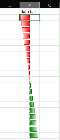
Conditional Formatting All Cells Data Bar

You can make a lot of different cool stuff with the data bar, lots of flexibility there.

Conditional Formatting Based On Numbers

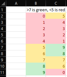
Pay attention to the dictionary inside the ws.conditional_format method, especially what values are passed into those properties. The ‘criteria’ can be any of the following (either column will work):

Conditional Formatting Based On Numbers From Cell Input

This is similar to the previous example, except that we are not hardcoding the threshold values 5 and 7. We will let the formatting depends on cell values – even more dynamic!

Pay close attention to the ‘ value’ property in the code below – we need to use absolute references, or it won’t work. In general, for any ‘value’ property we need to use an absolute reference.

Once we generate this in Excel, you’ll see that the formatting will change as we modify the values inside cells B19 and C19.

', 'value': '$B$19', 'format':format_g >) ws.conditional_format('B20:C29', ) 

Conditional Formatting Based On Text

• ‘containing’
• ‘not containing’
• ‘begins with’
• ‘ends with’

) ws.conditional_format('F2:F11', )

Conditional Formatting Top/Bottom Ranked Values

We can highlight the items by ‘top’ or ‘bottom’ values, i.e. first 5 largest, or by percent, i.e. bottom 10% of the selected values. Omitting the ‘criteria’ means by count, while setting ‘criteria’ : ‘%’ means by percentage.

Conditional Formatting Above/Below Average

For this one, Excel will calculate an average for the selected range, then compare each number in the range with the average, and format accordingly.

Conditional Formatting Unique/Duplicate Values

We can also highlight duplicated (or unique) values in a selected range.

Conditional Formatting Based On Formula

We can also do conditional formatting based on a formula – and make our Excel even much more dynamic!!

However, formula-based formatting can be a little bit tricky to work with because some situations require absolute references while others require a non-absolute reference. My go-to strategy is: try the formula in Excel, with or without $ in your cell references. If it works in your Excel, taking the same formula over to Python will also work.

The below code compares numbers in column R and column S, then highlights (in green) the larger number between the two columns.

Note that ‘type’ is set to ‘formula’ , in the ‘criteria’ we type the formula as if for the first item (of the selected range) only. Inside the conditional_format method, we are formatting cells R2:R11, the first element is R2, thus the formula is ‘=R2>S2’ . If we want to apply the format to R3:R11, then the formula needs to be ‘=R3>S3’, etc.

Also, note that in this case, we are comparing two columns so we don’t use absolute references in the formula. In other cases, you might need to use absolute references to make this formula-based formatting work. See my go-to strategy above.

S2', 'format':format_g >) ws.conditional_format('S2:S11', R2', 'format':format_g >)

That’s it! Leave a comment below if you need help with any specific scenario.

Источник

Python XlsxWriter — Conditional Formatting

Excel uses conditional formatting to change the appearance of cells in a range based on user defined criteria. From the conditional formatting menu, it is possible to define criteria involving various types of values.

In the worksheet shown below, the column A has different numbers. Numbers less than 50 are shown in red font color and grey background color.

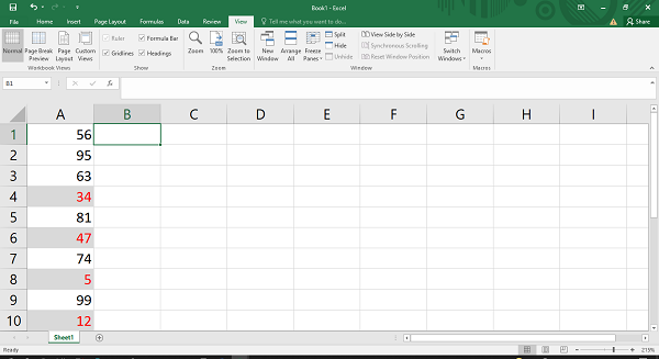
This is achieved by defining a conditional formatting rule below −

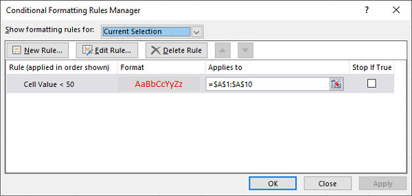
The conditional_format() method

In XlsxWriter, there as a conditional_format() method defined in the Worksheet class. To achieve the above shown result, the conditional_format() method is called as in the following code −

import xlsxwriter wb = xlsxwriter.Workbook('hello.xlsx') ws = wb.add_worksheet() data=[56,95,63,34,81,47,74,5,99,12] row=0 for num in data: ws.write(row,0,num) row+=1 f1 = wb.add_format() ws.conditional_format( 'A1:A10', < 'type':'cell', 'criteria':') wb.close()

Parameters

The conditional_format() method's first argument is the cell range, and the second argument is a dictionary of conditional formatting options.

The options dictionary configures the conditional formatting rules with the following parameters −

The type option is a required parameter. Its value is either cell, date, text, formula, etc. Each parameter has sub-parameters such as criteria, value, format, etc.

Type is the most common conditional formatting type. It is used when a format is applied to a cell based on a simple criterion.

The date type is similar the cell type and uses the same criteria and values. However, the value parameter should be given as a datetime object.

The text type specifies Excel's "Specific Text" style conditional format. It is used to do simple string matching using the criteria and value parameters.

Example

When formula type is used, the conditional formatting depends on a user defined formula.

import xlsxwriter wb = xlsxwriter.Workbook('hello.xlsx') ws = wb.add_worksheet() data = [ ['Anil', 45, 55, 50], ['Ravi', 60, 70, 80], ['Kiran', 65, 75, 85], ['Karishma', 55, 65, 45] ] for row in range(len(data)): ws.write_row(row,0, data[row]) f1 = wb.add_format() ws.conditional_format( 'A1:D4', < 'type':'formula', 'criteria':'=AVERAGE($B1:$D1)>60', 'value':50, 'format':f1 >) wb.close()

Output

Open the resultant workbook using MS Excel. We can see the rows satisfying the above condition displayed in blue color according to the format object. The conditional format rule manager also shows the criteria that we have set in the above code.

Источник