scipy.stats.norm#
The location ( loc ) keyword specifies the mean. The scale ( scale ) keyword specifies the standard deviation.
As an instance of the rv_continuous class, norm object inherits from it a collection of generic methods (see below for the full list), and completes them with details specific for this particular distribution.
The probability density function for norm is:
The probability density above is defined in the “standardized” form. To shift and/or scale the distribution use the loc and scale parameters. Specifically, norm.pdf(x, loc, scale) is identically equivalent to norm.pdf(y) / scale with y = (x — loc) / scale . Note that shifting the location of a distribution does not make it a “noncentral” distribution; noncentral generalizations of some distributions are available in separate classes.
>>> import numpy as np >>> from scipy.stats import norm >>> import matplotlib.pyplot as plt >>> fig, ax = plt.subplots(1, 1)
Calculate the first four moments:
>>> mean, var, skew, kurt = norm.stats(moments='mvsk')
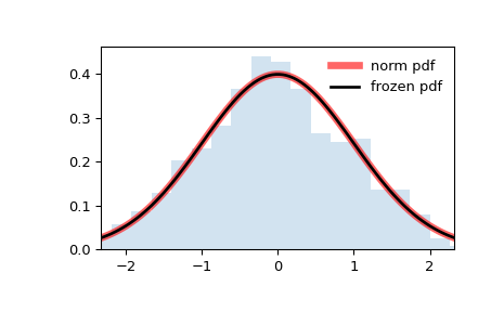
Display the probability density function ( pdf ):
>>> x = np.linspace(norm.ppf(0.01), . norm.ppf(0.99), 100) >>> ax.plot(x, norm.pdf(x), . 'r-', lw=5, alpha=0.6, label='norm pdf')
Alternatively, the distribution object can be called (as a function) to fix the shape, location and scale parameters. This returns a “frozen” RV object holding the given parameters fixed.
Freeze the distribution and display the frozen pdf :
>>> rv = norm() >>> ax.plot(x, rv.pdf(x), 'k-', lw=2, label='frozen pdf')
Check accuracy of cdf and ppf :
>>> vals = norm.ppf([0.001, 0.5, 0.999]) >>> np.allclose([0.001, 0.5, 0.999], norm.cdf(vals)) True
And compare the histogram:
>>> ax.hist(r, density=True, bins='auto', histtype='stepfilled', alpha=0.2) >>> ax.set_xlim([x[0], x[-1]]) >>> ax.legend(loc='best', frameon=False) >>> plt.show()
rvs(loc=0, scale=1, size=1, random_state=None)
pdf(x, loc=0, scale=1)
Probability density function.
logpdf(x, loc=0, scale=1)
Log of the probability density function.
cdf(x, loc=0, scale=1)
Cumulative distribution function.
logcdf(x, loc=0, scale=1)
Log of the cumulative distribution function.
sf(x, loc=0, scale=1)
Survival function (also defined as 1 — cdf , but sf is sometimes more accurate).
logsf(x, loc=0, scale=1)
Log of the survival function.
ppf(q, loc=0, scale=1)
Percent point function (inverse of cdf — percentiles).
isf(q, loc=0, scale=1)
Inverse survival function (inverse of sf ).
moment(order, loc=0, scale=1)
Non-central moment of the specified order.
stats(loc=0, scale=1, moments=’mv’)
Mean(‘m’), variance(‘v’), skew(‘s’), and/or kurtosis(‘k’).
entropy(loc=0, scale=1)
(Differential) entropy of the RV.
Parameter estimates for generic data. See scipy.stats.rv_continuous.fit for detailed documentation of the keyword arguments.
expect(func, args=(), loc=0, scale=1, lb=None, ub=None, conditional=False, **kwds)
Expected value of a function (of one argument) with respect to the distribution.
median(loc=0, scale=1)
Median of the distribution.
mean(loc=0, scale=1)
var(loc=0, scale=1)
Variance of the distribution.
std(loc=0, scale=1)
Standard deviation of the distribution.
interval(confidence, loc=0, scale=1)
Confidence interval with equal areas around the median.
Как рассчитать и построить нормальный CDF в Python
Кумулятивная функция распределения ( CDF ) говорит нам о вероятности того, что случайная величина примет значение, меньшее или равное некоторому значению.
В этом руководстве объясняется, как рассчитать и построить значения для обычного CDF в Python.
Пример 1. Расчет нормальных вероятностей CDF в Python
Самый простой способ рассчитать нормальные вероятности CDF в Python — использовать функцию norm.cdf() из библиотеки SciPy .
Следующий код показывает, как вычислить вероятность того, что случайная величина примет значение меньше 1,96 при стандартном нормальном распределении:
from scipy. stats import norm #calculate probability that random value is less than 1.96 in normal CDF norm. cdf ( 1.96 ) 0.9750021048517795 Вероятность того, что случайная величина примет значение меньше 1,96 при стандартном нормальном распределении, составляет примерно 0,975 .
Мы также можем найти вероятность того, что случайная величина примет значение больше 1,96, просто вычитая это значение из 1:
from scipy. stats import norm #calculate probability that random value is greater than 1.96 in normal CDF 1 - norm. cdf ( 1.96 ) 0.024997895148220484 Вероятность того, что случайная величина примет значение больше 1,96 при стандартном нормальном распределении, составляет примерно 0,025 .
Пример 2: Постройте нормальный CDF
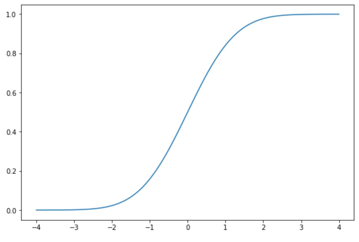
Следующий код показывает, как построить обычный CDF в Python:
import matplotlib.pyplot as plt import numpy as np import scipy. stats as ss #define x and y values to use for CDF x = np.linspace (-4, 4, 1000) y = ss. norm.cdf (x) #plot normal CDF plt.plot (x, y) 
На оси x показаны значения случайной величины, которые соответствуют стандартному нормальному распределению, а на оси y показана вероятность того, что случайная величина примет значение, меньшее, чем значение, показанное на оси x.
Например, если мы посмотрим на x = 1,96, то увидим, что совокупная вероятность того, что x меньше 1,96, составляет примерно 0,975 .
Не стесняйтесь изменять цвета и метки осей обычного графика CDF:
import matplotlib.pyplot as plt import numpy as np import scipy. stats as ss #define x and y values to use for CDF x = np.linspace (-4, 4, 1000) y = ss. norm.cdf (x) #plot normal CDF plt.plot (x, y, color='red') plt.title('Normal CDF') plt.xlabel('x') plt.ylabel('CDF') 
Дополнительные ресурсы
В следующих руководствах объясняется, как выполнять другие распространенные операции в Python: