Polynomial and Spline interpolation
This example demonstrates how to approximate a function with polynomials up to degree degree by using ridge regression. We show two different ways given n_samples of 1d points x_i :
- PolynomialFeatures generates all monomials up to degree . This gives us the so called Vandermonde matrix with n_samples rows and degree + 1 columns:
[[1, x_0, x_0 ** 2, x_0 ** 3, . , x_0 ** degree], [1, x_1, x_1 ** 2, x_1 ** 3, . , x_1 ** degree], . ]
[[basis_1(x_0), basis_2(x_0), . ], [basis_1(x_1), basis_2(x_1), . ], . ]
This example shows that these two transformers are well suited to model non-linear effects with a linear model, using a pipeline to add non-linear features. Kernel methods extend this idea and can induce very high (even infinite) dimensional feature spaces.
# Author: Mathieu Blondel # Jake Vanderplas # Christian Lorentzen # Malte Londschien # License: BSD 3 clause import matplotlib.pyplot as plt import numpy as np from sklearn.linear_model import Ridge from sklearn.pipeline import make_pipeline from sklearn.preprocessing import PolynomialFeatures, SplineTransformer
We start by defining a function that we intend to approximate and prepare plotting it.
def f(x): """Function to be approximated by polynomial interpolation.""" return x * np.sin(x) # whole range we want to plot x_plot = np.linspace(-1, 11, 100)
To make it interesting, we only give a small subset of points to train on.
x_train = np.linspace(0, 10, 100) rng = np.random.RandomState(0) x_train = np.sort(rng.choice(x_train, size=20, replace=False)) y_train = f(x_train) # create 2D-array versions of these arrays to feed to transformers X_train = x_train[:, np.newaxis] X_plot = x_plot[:, np.newaxis]
Now we are ready to create polynomial features and splines, fit on the training points and show how well they interpolate.
# plot function lw = 2 fig, ax = plt.subplots() ax.set_prop_cycle( color=["black", "teal", "yellowgreen", "gold", "darkorange", "tomato"] ) ax.plot(x_plot, f(x_plot), linewidth=lw, label="ground truth") # plot training points ax.scatter(x_train, y_train, label="training points") # polynomial features for degree in [3, 4, 5]: model = make_pipeline(PolynomialFeatures(degree), Ridge(alpha=1e-3)) model.fit(X_train, y_train) y_plot = model.predict(X_plot) ax.plot(x_plot, y_plot, label=f"degree degree>") # B-spline with 4 + 3 - 1 = 6 basis functions model = make_pipeline(SplineTransformer(n_knots=4, degree=3), Ridge(alpha=1e-3)) model.fit(X_train, y_train) y_plot = model.predict(X_plot) ax.plot(x_plot, y_plot, label="B-spline") ax.legend(loc="lower center") ax.set_ylim(-20, 10) plt.show()
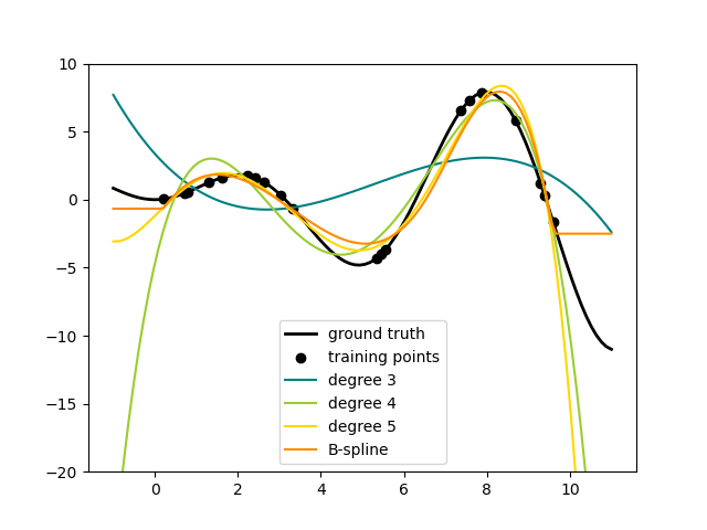
This shows nicely that higher degree polynomials can fit the data better. But at the same time, too high powers can show unwanted oscillatory behaviour and are particularly dangerous for extrapolation beyond the range of fitted data. This is an advantage of B-splines. They usually fit the data as well as polynomials and show very nice and smooth behaviour. They have also good options to control the extrapolation, which defaults to continue with a constant. Note that most often, you would rather increase the number of knots but keep degree=3 .
In order to give more insights into the generated feature bases, we plot all columns of both transformers separately.
fig, axes = plt.subplots(ncols=2, figsize=(16, 5)) pft = PolynomialFeatures(degree=3).fit(X_train) axes[0].plot(x_plot, pft.transform(X_plot)) axes[0].legend(axes[0].lines, [f"degree n>" for n in range(4)]) axes[0].set_title("PolynomialFeatures") splt = SplineTransformer(n_knots=4, degree=3).fit(X_train) axes[1].plot(x_plot, splt.transform(X_plot)) axes[1].legend(axes[1].lines, [f"spline n>" for n in range(6)]) axes[1].set_title("SplineTransformer") # plot knots of spline knots = splt.bsplines_[0].t axes[1].vlines(knots[3:-3], ymin=0, ymax=0.8, linestyles="dashed") plt.show()
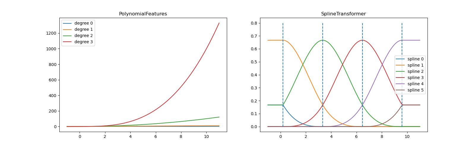
In the left plot, we recognize the lines corresponding to simple monomials from x**0 to x**3 . In the right figure, we see the six B-spline basis functions of degree=3 and also the four knot positions that were chosen during fit . Note that there are degree number of additional knots each to the left and to the right of the fitted interval. These are there for technical reasons, so we refrain from showing them. Every basis function has local support and is continued as a constant beyond the fitted range. This extrapolating behaviour could be changed by the argument extrapolation .
Periodic Splines
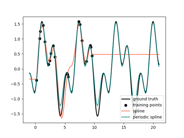
In the previous example we saw the limitations of polynomials and splines for extrapolation beyond the range of the training observations. In some settings, e.g. with seasonal effects, we expect a periodic continuation of the underlying signal. Such effects can be modelled using periodic splines, which have equal function value and equal derivatives at the first and last knot. In the following case we show how periodic splines provide a better fit both within and outside of the range of training data given the additional information of periodicity. The splines period is the distance between the first and last knot, which we specify manually.
Periodic splines can also be useful for naturally periodic features (such as day of the year), as the smoothness at the boundary knots prevents a jump in the transformed values (e.g. from Dec 31st to Jan 1st). For such naturally periodic features or more generally features where the period is known, it is advised to explicitly pass this information to the SplineTransformer by setting the knots manually.
def g(x): """Function to be approximated by periodic spline interpolation.""" return np.sin(x) - 0.7 * np.cos(x * 3) y_train = g(x_train) # Extend the test data into the future: x_plot_ext = np.linspace(-1, 21, 200) X_plot_ext = x_plot_ext[:, np.newaxis] lw = 2 fig, ax = plt.subplots() ax.set_prop_cycle(color=["black", "tomato", "teal"]) ax.plot(x_plot_ext, g(x_plot_ext), linewidth=lw, label="ground truth") ax.scatter(x_train, y_train, label="training points") for transformer, label in [ (SplineTransformer(degree=3, n_knots=10), "spline"), ( SplineTransformer( degree=3, knots=np.linspace(0, 2 * np.pi, 10)[:, None], extrapolation="periodic", ), "periodic spline", ), ]: model = make_pipeline(transformer, Ridge(alpha=1e-3)) model.fit(X_train, y_train) y_plot_ext = model.predict(X_plot_ext) ax.plot(x_plot_ext, y_plot_ext, label=label) ax.legend() fig.show()
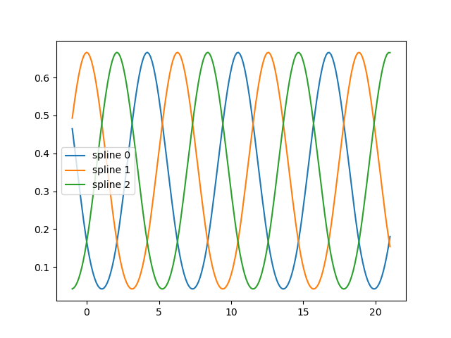
fig, ax = plt.subplots() knots = np.linspace(0, 2 * np.pi, 4) splt = SplineTransformer(knots=knots[:, None], degree=3, extrapolation="periodic").fit( X_train ) ax.plot(x_plot_ext, splt.transform(X_plot_ext)) ax.legend(ax.lines, [f"spline n>" for n in range(3)]) plt.show()
Total running time of the script: ( 0 minutes 0.469 seconds)
Простая программа на Python для гиперболической аппроксимации статистических данных
Законы Зипфа оописывают закономерности частотного распределения слов в тексте на любом естественном языке[1]. Эти законы кроме лингвистики применяться также в экономике [2]. Для аппроксимации статистических данных для объектов, которые подчиниться Законам Зипфа используется гиперболическая функция вида:
(1)
где: a.b – постоянные коэффициенты: x – статистические данные аргумента функции (в виде списка): y- приближение значений функции к реальным данным полученным методом наименьших квадратов[3].
Обычно для аппроксимации гиперболической функцией методом логарифмирования её приводят к линейной, а затем определяют коэффициенты a,b и делают обратное преобразование [4]. Прямое и обратное преобразование приводит к дополнительной погрешности аппроксимации. Поэтому привожу простую программу на Python, для классической реализации метода наименьших квадратов.
Алгоритм
Исходные данные задаются двумя списками где n ─ количество данных в списках.

Получим функцию для определения коэффициентов

Коэффициенты a,b найдём из следующей системы уравнений:(3)
Решение такой системы не представляет особого труда:
 (4),
(4),  (5).
(5).
Средняя ошибка аппроксимации  по формуле:
 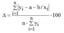 (6)
(6)
Код Python
#!/usr/bin/python # -*- coding: utf-8 -* import matplotlib.pyplot as plt import matplotlib as mpl mpl.rcParams['font.family'] = 'fantasy' def mnkGP(x,y): # функция которую можно использзовать в програме n=len(x) # количество элементов в списках s=sum(y) # сумма значений y s1=sum([1/x[i] for i in range(0,n)]) # сумма 1/x s2=sum([(1/x[i])**2 for i in range(0,n)]) # сумма (1/x)**2 s3=sum([y[i]/x[i] for i in range(0,n)]) # сумма y/x a= round((s*s2-s1*s3)/(n*s2-s1**2),3) # коэфициент а с тремя дробными цифрами b=round((n*s3-s1*s)/(n*s2-s1**2),3)# коэфициент b с тремя дробными цифрами s4=[a+b/x[i] for i in range(0,n)] # список значений гиперболической функции so=round(sum([abs(y[i] -s4[i]) for i in range(0,n)])/(n*sum(y))*100,3) # средняя ошибка аппроксимации plt.title('Аппроксимация гиперболой Y='+str(a)+'+'+str(b)+'/x\n Средняя ошибка--'+str(so)+'%',size=14) plt.xlabel('Координата X', size=14) plt.ylabel('Координата Y', size=14) plt.plot(x, y, color='r', linestyle=' ', marker='o', label='Data(x,y)') plt.plot(x, s4, color='g', linewidth=2, label='Data(x,f(x)=a+b/x') plt.legend(loc='best') plt.grid(True) plt.show() x=[10, 14, 18, 22, 26, 30, 34, 38, 42, 46, 50, 54, 58, 62, 66, 70, 74, 78, 82, 86] y=[0.1, 0.0714, 0.0556, 0.0455, 0.0385, 0.0333, 0.0294, 0.0263, 0.0238, 0.0217, 0.02, 0.0185, 0.0172, 0.0161, 0.0152, 0.0143, 0.0135, 0.0128, 0.0122, 0.0116] # данные для проверки по функции y=1/x mnkGP(x,y) Результат
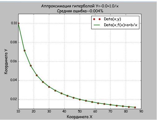
Мы брали данные из функции равносторонней гиперболы, поэтому и получили a=0,b=10 и абсолютную погрешность в 0,004%. Значить функция mnkGP(x,y) работает правильно и её можно вставлять в прикладную программу
Аппроксимация для степенных функций
Для этого в Python есть модуль scipy, но он не поддерживает отрицательную степень d полинома. Рассмотрим код реализации аппроксимации данных полиномом.
#!/usr/bin/python # coding: utf8 import scipy as sp import matplotlib.pyplot as plt def mnkGP(x,y): d=2 # степень полинома fp, residuals, rank, sv, rcond = sp.polyfit(x, y, d, full=True) # Модель f = sp.poly1d(fp) # аппроксимирующая функция print('Коэффициент -- a %s '%round(fp[0],4)) print('Коэффициент-- b %s '%round(fp[1],4)) print('Коэффициент -- c %s '%round(fp[2],4)) y1=[fp[0]*x[i]**2+fp[1]*x[i]+fp[2] for i in range(0,len(x))] # значения функции a*x**2+b*x+c so=round(sum([abs(y[i]-y1[i]) for i in range(0,len(x))])/(len(x)*sum(y))*100,4) # средняя ошибка print('Average quadratic deviation '+str(so)) fx = sp.linspace(x[0], x[-1] + 1, len(x)) # можно установить вместо len(x) большее число для интерполяции plt.plot(x, y, 'o', label='Original data', markersize=10) plt.plot(fx, f(fx), linewidth=2) plt.grid(True) plt.show() x=[10, 14, 18, 22, 26, 30, 34, 38, 42, 46, 50, 54, 58, 62, 66, 70, 74, 78, 82, 86] y=[0.1, 0.0714, 0.0556, 0.0455, 0.0385, 0.0333, 0.0294, 0.0263, 0.0238, 0.0217, 0.02, 0.0185, 0.0172, 0.0161, 0.0152, 0.0143, 0.0135, 0.0128, 0.0122, 0.0116] # данные для проверки по функции y=1/x mnkGP(x,y) Результат

Как следует из графика, при аппроксимации параболой данных изменяющихся по гиперболе средняя ошибка возрастает, а свободный член квадратного уравнения обращается в ноль.
Полученные функции будут применены для анализа Законов Зипфа (Ципфа), но это будет сделано уже в следующей статье.