3д пончик код python

Basics of Donut charts with Python’s Matplotlib

A quick guide on different ways to plot a donut with Matplotlib

With many similarities to pie charts, this creative visualization sets itself apart from its infamous cousin. The open center makes the slices look like bars and change the focus of the comparison from areas and angles to the length.

In this article, we’ll check two ways of plotting donut charts with Matplolib. A simple approach with Pie charts and the parameter wedgeprops, and a more complex method with polar axis and horizontal bar charts.

Pies

There’s no method for drawing a donut chart in Matplotlib, but we can quickly transform a Pie chart with wedgeprops.

Let’s start with a simple pie.

import matplotlib.pyplot as pltplt.pie([87,13], startangle=90, colors=['#5DADE2', '#515A5A'])plt.show()

Now we can add the parameter wedgeprops and define the width of the edges, where one means the border will go all the way to the center.

fig, ax = plt.subplots(figsize=(6, 6)) 

ax.pie([87,13], 
wedgeprops=, 
startangle=90, 
colors=['#5DADE2', '#515A5A'])plt.show()

That’s very straightforward. And now that we can use the space at the center to make our data even more evident.

fig, ax = plt.subplots(figsize=(6, 6))wedgeprops = ax.pie([87,13], wedgeprops=wedgeprops, startangle=90, colors=['#5DADE2', '#515A5A'])plt.title('Worldwide Access to Electricity', fontsize=24, loc='left')plt.text(0, 0, "87%", ha='center', va='center', fontsize=42)
plt.text(-1.2, -1.2, "Source: ourworldindata.org/energy-access", ha='left', va='center'…

Источник

Denbergvanthijs / donut.py

This file contains bidirectional Unicode text that may be interpreted or compiled differently than what appears below. To review, open the file in an editor that reveals hidden Unicode characters. Learn more about bidirectional Unicode characters

import numpy as np

screen_size = 40

theta_spacing = 0.07

phi_spacing = 0.02

illumination = np . fromiter ( «.,-~:;=!*#$@» , dtype = »

A = 1

B = 1

R1 = 1

R2 = 2

K2 = 5

K1 = screen_size * K2 * 3 / ( 8 * ( R1 + R2 ))

def render_frame ( A : float , B : float ) -> np . ndarray :

«»»

Returns a frame of the spinning 3D donut.

Based on the pseudocode from: https://www.a1k0n.net/2011/07/20/donut-math.html

«»»

cos_A = np . cos ( A )

sin_A = np . sin ( A )

cos_B = np . cos ( B )

sin_B = np . sin ( B )

output = np . full (( screen_size , screen_size ), » » ) # (40, 40)

zbuffer = np . zeros (( screen_size , screen_size )) # (40, 40)

cos_phi = np . cos ( phi := np . arange ( 0 , 2 * np . pi , phi_spacing )) # (315,)

sin_phi = np . sin ( phi ) # (315,)

cos_theta = np . cos ( theta := np . arange ( 0 , 2 * np . pi , theta_spacing )) # (90,)

sin_theta = np . sin ( theta ) # (90,)

circle_x = R2 + R1 * cos_theta # (90,)

circle_y = R1 * sin_theta # (90,)

x = ( np . outer ( cos_B * cos_phi + sin_A * sin_B * sin_phi , circle_x ) — circle_y * cos_A * sin_B ). T # (90, 315)

y = ( np . outer ( sin_B * cos_phi — sin_A * cos_B * sin_phi , circle_x ) + circle_y * cos_A * cos_B ). T # (90, 315)

z = (( K2 + cos_A * np . outer ( sin_phi , circle_x )) + circle_y * sin_A ). T # (90, 315)

ooz = np . reciprocal ( z ) # Calculates 1/z

xp = ( screen_size / 2 + K1 * ooz * x ). astype ( int ) # (90, 315)

yp = ( screen_size / 2 — K1 * ooz * y ). astype ( int ) # (90, 315)

L1 = ((( np . outer ( cos_phi , cos_theta ) * sin_B ) — cos_A * np . outer ( sin_phi , cos_theta )) — sin_A * sin_theta ) # (315, 90)

L2 = cos_B * ( cos_A * sin_theta — np . outer ( sin_phi , cos_theta * sin_A )) # (315, 90)

L = np . around ((( L1 + L2 ) * 8 )). astype ( int ). T # (90, 315)

mask_L = L >= 0 # (90, 315)

chars = illumination [ L ] # (90, 315)

for i in range ( 90 ):

mask = mask_L [ i ] & ( ooz [ i ] > zbuffer [ xp [ i ], yp [ i ]]) # (315,)

zbuffer [ xp [ i ], yp [ i ]] = np . where ( mask , ooz [ i ], zbuffer [ xp [ i ], yp [ i ]])

output [ xp [ i ], yp [ i ]] = np . where ( mask , chars [ i ], output [ xp [ i ], yp [ i ]])

return output

def pprint ( array : np . ndarray ) -> None :

«»»Pretty print the frame.»»»

print ( * [ » » . join ( row ) for row in array ], sep = » \n » )

if __name__ == «__main__» :

for _ in range ( screen_size * screen_size ):

A += theta_spacing

B += phi_spacing

print ( » \x1b [H» )

pprint ( render_frame ( A , B ))

Источник

Donut Plot

A Donut chart is essentially a Pie Chart with an area of the center cut out. You can build one hacking the plt.pie() function of the matplotlib library as shown in the examples below.

⏱ Quick start

matplotlib allows to build a pie chart easily thanks to its pie() function. Visit the dedicated section for more about that.

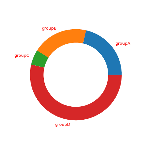
We can use the exact same principle and add a circle to the center thanks to the circle() function and get a donut chart.🔥

Most basic donut chart with Python and Matplotlib

# library import matplotlib.pyplot as plt # create data size_of_groups=[12,11,3,30] # Create a pieplot plt.pie(size_of_groups) # add a circle at the center to transform it in a donut chart my_circle=plt.Circle( (0,0), 0.7, color='white') p=plt.gcf() p.gca().add_artist(my_circle) plt.show() 

⚠️ Mind the donut!

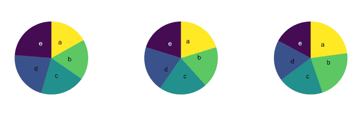
As his friend the Pie chart, the Donut chart is often criticized. Humans are pretty bad at reading angles, making it hard to rank the groups accurately. Most of the time, it is better to display the information as a barchart, a treemap or a lollipop plot.

Have a look to the 3 pie charts below, can you spot the pattern hidden in it?

The matplotlib-venn library allows a high level of customization. Here is an example taking advantage of it

Donut plot with Matplotlib

The example above is a good start but you probably need to go further. The blog posts linked below explain common tasks like adding and customizing labels, change section colors, add padding between each and more.

Add and customize the labels

Источник

Подборка неожиданного, странного, местами безумного кода: самые необычные программы из когда-либо написанных

Сегодня мы поговорим о самых странных программах, какие вы когда-либо видели. Настолько странных, что они сломают ваш мозг. Настолько маленьких, что не верится, что они работают. И настолько непонятных, что даже прошаренные кодеры начнут неистово гуглить.

Примечание Никогда не используйте такой код в реальных проектах — читаемость и поддерживаемость превыше всего.

Уровень 0. Вступление

Взгляните на этот милый код:

Это регулярное выражение написано на Perl и проверяет, является ли число простым. Вот полный код программы для запуска. А вот наше руководство по Perl, чтобы вы могли начать его изучать.

А это выражение выдаст день недели для заданной даты:

А как вам этот код на Java?

int i = (byte) + (char) - (int) + (long) - 1;

Чему будет равно i ? Он вообще скомпилируется? Да уж…

А программа на гифке ниже — это куайн по имени qlobe, написанный на Ruby. Ну разве это не изумительно?

А эта — ну просто шедевр! Анимированный 3D-пончик, какая вкуснятина!

Вставьте этот код в адресную строку:

data:text/html,

и оцените всю магию самостоятельно!

Tech Lead/Senior Python developer на продукт Data Quality (DataOps Platform) МТС , Москва, можно удалённо , По итогам собеседования

А вообще лучше ничего не копипастьте, особенно код для командной строки, последствия могут быть неприятными.

Большую часть программ, приведённых ниже, вы вряд ли поймёте. Но описания по ссылкам помогут прояснить ситуацию. Для запуска этих программ вам может понадобится один из онлайн-компиляторов, о которых мы рассказывали в одной из наших статей, например, ресурсы TutorialsPoint-CodingGround и repl.it — там есть онлайн-редакторы кода и компиляторы.

Источник